---
title: "模型构建"
subtitle: 《区域水环境污染数据分析实践》
Data analysis practice of regional water environment pollution
author: 苏命、王为东
中国科学院大学资源与环境学院
中国科学院生态环境研究中心
date: today
lang: zh
format:
revealjs:
theme: dark
slide-number: true
chalkboard:
buttons: true
preview-links: auto
lang: zh
toc: true
toc-depth: 1
toc-title: 大纲
logo: ./_extensions/inst/img/ucaslogo.png
css: ./_extensions/inst/css/revealjs.css
pointer:
key: "p"
color: "#32cd32"
pointerSize: 18
revealjs-plugins:
- pointer
filters:
- d2
knitr:
opts_chunk:
dev: "svg"
retina: 3
execute:
freeze: auto
cache: true
echo: true
fig-width: 5
fig-height: 6
---
# tidymodels主要步骤
```{r}
#| echo: false
hexes <- function(..., size = 64) {
x <- c(...)
x <- sort(unique(x), decreasing = TRUE)
right <- (seq_along(x) - 1) * size
res <- glue::glue(
'{.absolute top=-20 right= width="" height=""}',
.open = "<", .close = ">"
)
paste0(res, collapse = " ")
}
knitr::opts_chunk$set(
digits = 3,
comment = "#>",
dev = 'svglite'
)
# devtools::install_github("gadenbuie/countdown")
# library(countdown)
library(ggplot2)
theme_set(theme_bw())
options(cli.width = 70, ggplot2.discrete.fill = c("#7e96d5", "#de6c4e"))
train_color <- "#1a162d"
test_color <- "#cd4173"
data_color <- "#767381"
assess_color <- "#84cae1"
splits_pal <- c(data_color, train_color, test_color)
```
## 何为tidymodels? {background-image="images/tm-org.png" background-size="80%"}
```{r load-tm}
#| message: true
#| echo: true
#| warning: true
library(tidymodels)
```
## 整体思路
```{r diagram-split, echo = FALSE}
#| fig-align: "center"
knitr::include_graphics("images/whole-game-split.jpg")
```
## 整体思路
```{r diagram-model-1, echo = FALSE}
#| fig-align: "center"
knitr::include_graphics("images/whole-game-model-1.jpg")
```
:::notes
Stress that we are **not** fitting a model on the entire training set other than for illustrative purposes in deck 2.
:::
## 整体思路
```{r diagram-model-n, echo = FALSE}
#| fig-align: "center"
knitr::include_graphics("images/whole-game-model-n.jpg")
```
## 整体思路
```{r, echo = FALSE}
#| fig-align: "center"
knitr::include_graphics("images/whole-game-resamples.jpg")
```
## 整体思路
```{r, echo = FALSE}
#| fig-align: "center"
knitr::include_graphics("images/whole-game-select.jpg")
```
## 整体思路
```{r diagram-final-fit, echo = FALSE}
#| fig-align: "center"
knitr::include_graphics("images/whole-game-final-fit.jpg")
```
## 整体思路
```{r diagram-final-performance, echo = FALSE}
#| fig-align: "center"
knitr::include_graphics("images/whole-game-final-performance.jpg")
```
## 相关包的安装
```{r load-pkgs}
#| eval: false
# Install the packages for the workshop
pkgs <-
c("bonsai", "doParallel", "embed", "finetune", "lightgbm", "lme4",
"plumber", "probably", "ranger", "rpart", "rpart.plot", "rules",
"splines2", "stacks", "text2vec", "textrecipes", "tidymodels",
"vetiver", "remotes")
install.packages(pkgs)
```
. . .
## Data on Chicago taxi trips
```{r taxi-print}
library(tidymodels)
taxi
```
## 数据分割与使用
对于机器学习,我们通常将数据分成训练集和测试集:
. . .
- 训练集用于估计模型参数。
- 测试集用于独立评估模型性能。
. . .
在训练过程中不要使用测试集。
. . .
```{r test-train-split}
#| echo: false
#| fig.width: 12
#| fig.height: 3
#|
set.seed(123)
library(forcats)
one_split <- slice(taxi, 1:30) %>%
initial_split() %>%
tidy() %>%
add_row(Row = 1:30, Data = "Original") %>%
mutate(Data = case_when(
Data == "Analysis" ~ "Training",
Data == "Assessment" ~ "Testing",
TRUE ~ Data
)) %>%
mutate(Data = factor(Data, levels = c("Original", "Training", "Testing")))
all_split <-
ggplot(one_split, aes(x = Row, y = fct_rev(Data), fill = Data)) +
geom_tile(color = "white",
linewidth = 1) +
scale_fill_manual(values = splits_pal, guide = "none") +
theme_minimal() +
theme(axis.text.y = element_text(size = rel(2)),
axis.text.x = element_blank(),
legend.position = "top",
panel.grid = element_blank()) +
coord_equal(ratio = 1) +
labs(x = NULL, y = NULL)
all_split
```
## The initial split
```{r taxi-split}
set.seed(123)
taxi_split <- initial_split(taxi)
taxi_split
```
## Accessing the data
```{r taxi-train-test}
taxi_train <- training(taxi_split)
taxi_test <- testing(taxi_split)
```
## The training set
```{r taxi-train}
taxi_train
```
## 练习
```{r taxi-split-prop}
set.seed(123)
taxi_split <- initial_split(taxi, prop = 0.8)
taxi_train <- training(taxi_split)
taxi_test <- testing(taxi_split)
nrow(taxi_train)
nrow(taxi_test)
```
## Stratification
Use `strata = tip`
```{r taxi-split-prop-strata}
set.seed(123)
taxi_split <- initial_split(taxi, prop = 0.8, strata = tip)
taxi_split
```
## Stratification
Stratification often helps, with very little downside
```{r taxi-tip-pct-by-split, echo = FALSE}
bind_rows(
taxi_train %>% mutate(split = "train"),
taxi_test %>% mutate(split = "test")
) %>%
ggplot(aes(x = split, fill = tip)) +
geom_bar(position = "fill")
```
## 模型类型
模型多种多样
- `lm` for linear model
- `glm` for generalized linear model (e.g. logistic regression)
- `glmnet` for regularized regression
- `keras` for regression using TensorFlow
- `stan` for Bayesian regression
- `spark` for large data sets
## 指定模型
```{r}
#| echo: false
library(tidymodels)
set.seed(123)
taxi_split <- initial_split(taxi, prop = 0.8, strata = tip)
taxi_train <- training(taxi_split)
taxi_test <- testing(taxi_split)
```
```{r logistic-reg}
logistic_reg()
```
:::notes
Models have default engines
:::
## To specify a model
```{r logistic-reg-glmnet}
logistic_reg() %>%
set_engine("glmnet")
```
. . .
```{r logistic-reg-stan}
logistic_reg() %>%
set_engine("stan")
```
::: columns
::: {.column width="40%"}
- Choose a model
- Specify an engine
- Set the [mode]{.underline}
:::
::: {.column width="60%"}

:::
:::
## To specify a model
```{r decision-tree}
decision_tree()
```
:::notes
Some models have a default mode
:::
## To specify a model
```{r decision-tree-classification}
decision_tree() %>%
set_mode("classification")
```
. . .
::: r-fit-text
All available models are listed at
:::
## Workflows
```{r good-workflow}
#| echo: false
#| out-width: '70%'
#| fig-align: 'center'
knitr::include_graphics("images/good_workflow.png")
```
## 为什么要使用 `workflow()`?
- 与基本的 R 工具相比,工作流能更好地处理新的因子水平
. . .
- 除了公式之外,还可以使用其他的预处理器(更多关于高级 tidymodels 中的特征工程!)
. . .
- 在使用多个模型时,它们可以帮助组织工作
. . .
- [最重要的是]{.underline},工作流涵盖了整个建模过程:`fit()` 和 `predict()` 不仅适用于实际的模型拟合,还适用于预处理步骤
::: notes
工作流比基本的 R 处理水平更好的两种方式:
- 强制要求在预测时不允许出现新的水平(这是一个可选的检查,可以关闭)
- 恢复在拟合时存在但在预测时缺失的水平(例如,“新”数据中没有该水平的实例)
:::
## A model workflow
```{r tree-spec}
tree_spec <-
decision_tree(cost_complexity = 0.002) %>%
set_mode("classification")
tree_spec %>%
fit(tip ~ ., data = taxi_train)
```
## A model workflow
```{r tree-wflow}
tree_spec <-
decision_tree(cost_complexity = 0.002) %>%
set_mode("classification")
workflow() %>%
add_formula(tip ~ .) %>%
add_model(tree_spec) %>%
fit(data = taxi_train)
```
## A model workflow
```{r tree-wflow-fit}
tree_spec <-
decision_tree(cost_complexity = 0.002) %>%
set_mode("classification")
workflow(tip ~ ., tree_spec) %>%
fit(data = taxi_train)
```
## 预测
How do you use your new `tree_fit` model?
```{r tree-wflow-fit-2}
tree_spec <-
decision_tree(cost_complexity = 0.002) %>%
set_mode("classification")
tree_fit <-
workflow(tip ~ ., tree_spec) %>%
fit(data = taxi_train)
```
## 练习
*Run:*
`predict(tree_fit, new_data = taxi_test)`
. . .
*Run:*
`augment(tree_fit, new_data = taxi_test)`
*What do you get?*
## tidymodels 的预测
- 预测结果始终在一个 **tibble** 内
- 列名和类型可读性强
- `new_data` 中的行数和输出中的行数**相同**
## 理解模型
如何 **理解**`tree_fit` 模型?
```{r plot-tree-fit-4}
#| echo: false
#| fig-align: center
#| fig-width: 8
#| fig-height: 5
#| out-width: 100%
library(rpart.plot)
tree_fit %>%
extract_fit_engine() %>%
rpart.plot(roundint = FALSE)
```
## Evaluating models: 预测值
```{r}
#| echo: false
library(tidymodels)
set.seed(123)
taxi_split <- initial_split(taxi, prop = 0.8, strata = tip)
taxi_train <- training(taxi_split)
taxi_test <- testing(taxi_split)
tree_spec <- decision_tree(cost_complexity = 0.0001, mode = "classification")
taxi_wflow <- workflow(tip ~ ., tree_spec)
taxi_fit <- fit(taxi_wflow, taxi_train)
```
```{r taxi-fit-augment}
augment(taxi_fit, new_data = taxi_train) %>%
relocate(tip, .pred_class, .pred_yes, .pred_no)
```
## Confusion matrix
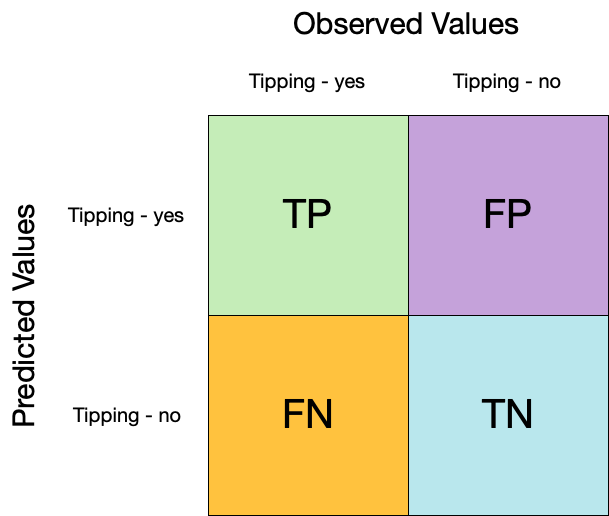
## Confusion matrix
```{r conf-mat}
augment(taxi_fit, new_data = taxi_train) %>%
conf_mat(truth = tip, estimate = .pred_class)
```
## Confusion matrix
```{r conf-mat-plot}
augment(taxi_fit, new_data = taxi_train) %>%
conf_mat(truth = tip, estimate = .pred_class) %>%
autoplot(type = "heatmap")
```
## Metrics for model performance
::: columns
::: {.column width="60%"}
```{r acc}
augment(taxi_fit, new_data = taxi_train) %>%
accuracy(truth = tip, estimate = .pred_class)
```
:::
::: {.column width="40%"}
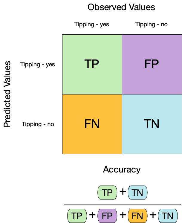
:::
:::
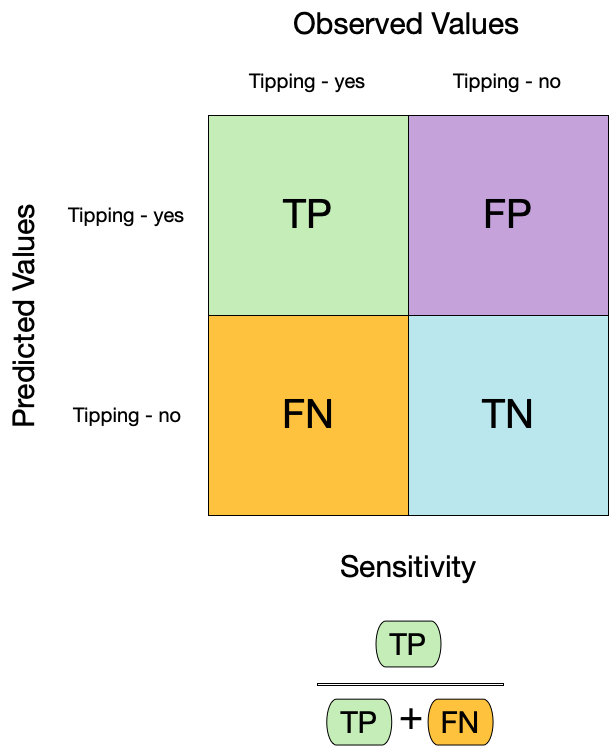
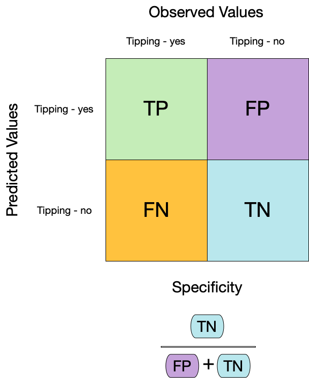
## 二分类模型评估
模型的敏感性(Sensitivity)和特异性(Specificity)是评估二分类模型性能的重要指标:
- **敏感性**(Sensitivity),也称为真阳性率,衡量了模型正确识别正类别样本的能力。公式为真阳性数除以真阳性数加上假阴性数:
$$
\text{Sensitivity} = \frac{\text{True Positives}}{\text{True Positives} + \text{False Negatives}}
$$
- **特异性**(Specificity),也称为真阴性率,衡量了模型正确识别负类别样本的能力。公式为真阴性数除以真阴性数加上假阳性数:
$$
\text{Specificity} = \frac{\text{True Negatives}}{\text{True Negatives} + \text{False Positives}}
$$
在评估模型时,我们希望敏感性和特异性都很高。高敏感性表示模型能够捕获真正的正类别样本,高特异性表示模型能够准确排除负类别样本。
## Metrics for model performance
::: columns
::: {.column width="60%"}
```{r sens}
augment(taxi_fit, new_data = taxi_train) %>%
sensitivity(truth = tip, estimate = .pred_class)
```
:::
::: {.column width="40%"}
:::
:::
## Metrics for model performance
::: columns
::: {.column width="60%"}
```{r sens-2}
#| code-line-numbers: "3-6"
augment(taxi_fit, new_data = taxi_train) %>%
sensitivity(truth = tip, estimate = .pred_class)
```
```{r spec}
augment(taxi_fit, new_data = taxi_train) %>%
specificity(truth = tip, estimate = .pred_class)
```
:::
::: {.column width="40%"}
:::
:::
## Metrics for model performance
We can use `metric_set()` to combine multiple calculations into one
```{r taxi-metrics}
taxi_metrics <- metric_set(accuracy, specificity, sensitivity)
augment(taxi_fit, new_data = taxi_train) %>%
taxi_metrics(truth = tip, estimate = .pred_class)
```
## Metrics for model performance
```{r taxi-metrics-grouped}
taxi_metrics <- metric_set(accuracy, specificity, sensitivity)
augment(taxi_fit, new_data = taxi_train) %>%
group_by(local) %>%
taxi_metrics(truth = tip, estimate = .pred_class)
```
## Varying the threshold
```{r}
#| label: thresholds
#| echo: false
augment(taxi_fit, new_data = taxi_train) %>%
roc_curve(truth = tip, .pred_yes) %>%
filter(is.finite(.threshold)) %>%
pivot_longer(c(specificity, sensitivity), names_to = "statistic", values_to = "value") %>%
rename(`event threshold` = .threshold) %>%
ggplot(aes(x = `event threshold`, y = value, col = statistic, group = statistic)) +
geom_line() +
scale_color_brewer(palette = "Dark2") +
labs(y = NULL) +
coord_equal() +
theme(legend.position = "top")
```
## ROC 曲线
- ROC(Receiver Operating Characteristic)曲线用于评估二分类模型的性能,特别是在不同的阈值下比较模型的敏感性和特异性。
- ROC曲线的横轴是假阳性率(False Positive Rate,FPR),纵轴是真阳性率(True Positive Rate,TPR)。在ROC曲线上,每个点对应于一个特定的阈值。通过改变阈值,我们可以观察到模型在不同条件下的表现。
- ROC曲线越接近左上角(0,1)点,说明模型的性能越好,因为这表示在较低的假阳性率下,模型能够获得较高的真阳性率。ROC曲线下面积(Area Under the ROC Curve,AUC)也是评估模型性能的一种指标,AUC值越大表示模型性能越好。
## ROC curve plot
```{r roc-curve}
#| fig-width: 6
#| fig-height: 6
#| output-location: "column"
augment(taxi_fit, new_data = taxi_train) %>%
roc_curve(truth = tip, .pred_yes) %>%
autoplot()
```
## 过度拟合

## 过度拟合

## Cross-validation {background-color="white" background-image="https://www.tmwr.org/premade/resampling.svg" background-size="80%"}
## Cross-validation

## Cross-validation

## Cross-validation
```{r vfold-cv}
vfold_cv(taxi_train) # v = 10 is default
```
## Cross-validation
What is in this?
```{r taxi-splits}
taxi_folds <- vfold_cv(taxi_train)
taxi_folds$splits[1:3]
```
::: notes
Talk about a list column, storing non-atomic types in dataframe
:::
## Cross-validation
```{r vfold-cv-v}
vfold_cv(taxi_train, v = 5)
```
## Cross-validation
```{r vfold-cv-strata}
vfold_cv(taxi_train, strata = tip)
```
. . .
Stratification often helps, with very little downside
## Cross-validation
We'll use this setup:
```{r taxi-folds}
set.seed(123)
taxi_folds <- vfold_cv(taxi_train, v = 10, strata = tip)
taxi_folds
```
. . .
Set the seed when creating resamples
## Fit our model to the resamples
```{r fit-resamples}
taxi_res <- fit_resamples(taxi_wflow, taxi_folds)
taxi_res
```
## Evaluating model performance
```{r collect-metrics}
taxi_res %>%
collect_metrics()
```
::: notes
collect_metrics() 是一套 collect_*() 函数之一,可用于处理调参结果的列。调参结果中以 . 为前缀的大多数列都有对应的 collect_*() 函数,可以进行常见摘要选项的汇总。
:::
. . .
We can reliably measure performance using only the **training** data 🎉
## Comparing metrics
How do the metrics from resampling compare to the metrics from training and testing?
```{r calc-roc-auc}
#| echo: false
taxi_training_roc_auc <-
taxi_fit %>%
augment(taxi_train) %>%
roc_auc(tip, .pred_yes) %>%
pull(.estimate) %>%
round(digits = 2)
taxi_testing_roc_auc <-
taxi_fit %>%
augment(taxi_test) %>%
roc_auc(tip, .pred_yes) %>%
pull(.estimate) %>%
round(digits = 2)
```
::: columns
::: {.column width="50%"}
```{r collect-metrics-2}
taxi_res %>%
collect_metrics() %>%
select(.metric, mean, n)
```
:::
::: {.column width="50%"}
The ROC AUC previously was
- `r taxi_training_roc_auc` for the training set
- `r taxi_testing_roc_auc` for test set
:::
:::
. . .
Remember that:
⚠️ the training set gives you overly optimistic metrics
⚠️ the test set is precious
## Evaluating model performance
```{r save-predictions}
# Save the assessment set results
ctrl_taxi <- control_resamples(save_pred = TRUE)
taxi_res <- fit_resamples(taxi_wflow, taxi_folds, control = ctrl_taxi)
taxi_res
```
## Evaluating model performance
```{r collect-predictions}
# Save the assessment set results
taxi_preds <- collect_predictions(taxi_res)
taxi_preds
```
## Evaluating model performance
```{r taxi-metrics-by-id}
taxi_preds %>%
group_by(id) %>%
taxi_metrics(truth = tip, estimate = .pred_class)
```
## Where are the fitted models?
```{r taxi-res}
taxi_res
```
## Bootstrapping

## Bootstrapping
```{r bootstraps}
set.seed(3214)
bootstraps(taxi_train)
```
## Monte Carlo Cross-Validation
```{r mc-cv}
set.seed(322)
mc_cv(taxi_train, times = 10)
```
## Validation set
```{r validation-split}
set.seed(853)
taxi_val_split <- initial_validation_split(taxi, strata = tip)
validation_set(taxi_val_split)
```
## Create a random forest model
```{r rf-spec}
rf_spec <- rand_forest(trees = 1000, mode = "classification")
rf_spec
```
## Create a random forest model
```{r rf-wflow}
rf_wflow <- workflow(tip ~ ., rf_spec)
rf_wflow
```
## Evaluating model performance
```{r collect-metrics-rf}
ctrl_taxi <- control_resamples(save_pred = TRUE)
# Random forest uses random numbers so set the seed first
set.seed(2)
rf_res <- fit_resamples(rf_wflow, taxi_folds, control = ctrl_taxi)
collect_metrics(rf_res)
```
## The whole game - status update
```{r diagram-select, echo = FALSE}
#| fig-align: "center"
knitr::include_graphics("images/whole-game-transparent-select.jpg")
```
## The final fit
```{r final-fit}
# taxi_split has train + test info
final_fit <- last_fit(rf_wflow, taxi_split)
final_fit
```
## 何为`final_fit`?
```{r collect-metrics-final-fit}
collect_metrics(final_fit)
```
. . .
These are metrics computed with the **test** set
## 何为`final_fit`?
```{r collect-predictions-final-fit}
collect_predictions(final_fit)
```
## 何为`final_fit`?
```{r extract-workflow}
extract_workflow(final_fit)
```
. . .
Use this for **prediction** on new data, like for deploying
## Tuning models - Specifying tuning parameters
```{r}
#| label: tag-for-tuning
#| code-line-numbers: "1|"
rf_spec <- rand_forest(min_n = tune()) %>%
set_mode("classification")
rf_wflow <- workflow(tip ~ ., rf_spec)
rf_wflow
```
## Try out multiple values
`tune_grid()` works similar to `fit_resamples()` but covers multiple parameter values:
```{r}
#| label: rf-tune_grid
#| code-line-numbers: "2|3-4|5|"
set.seed(22)
rf_res <- tune_grid(
rf_wflow,
taxi_folds,
grid = 5
)
```
## Compare results
Inspecting results and selecting the best-performing hyperparameter(s):
```{r}
#| label: rf-results
show_best(rf_res)
best_parameter <- select_best(rf_res)
best_parameter
```
`collect_metrics()` and `autoplot()` are also available.
## The final fit
```{r}
#| label: rf-finalize
rf_wflow <- finalize_workflow(rf_wflow, best_parameter)
final_fit <- last_fit(rf_wflow, taxi_split)
collect_metrics(final_fit)
```
# 实践部分
## 数据
```{r}
require(tidyverse)
sitedf <- readr::read_csv("https://www.epa.gov/sites/default/files/2014-01/nla2007_sampledlakeinformation_20091113.csv") |>
select(SITE_ID,
lon = LON_DD,
lat = LAT_DD,
name = LAKENAME,
area = LAKEAREA,
zmax = DEPTHMAX
) |>
group_by(SITE_ID) |>
summarize(lon = mean(lon, na.rm = TRUE),
lat = mean(lat, na.rm = TRUE),
name = unique(name),
area = mean(area, na.rm = TRUE),
zmax = mean(zmax, na.rm = TRUE))
visitdf <- readr::read_csv("https://www.epa.gov/sites/default/files/2013-09/nla2007_profile_20091008.csv") |>
select(SITE_ID,
date = DATE_PROFILE,
year = YEAR,
visit = VISIT_NO
) |>
distinct()
waterchemdf <- readr::read_csv("https://www.epa.gov/sites/default/files/2013-09/nla2007_profile_20091008.csv") |>
select(SITE_ID,
date = DATE_PROFILE,
depth = DEPTH,
temp = TEMP_FIELD,
do = DO_FIELD,
ph = PH_FIELD,
cond = COND_FIELD,
)
sddf <- readr::read_csv("https://www.epa.gov/sites/default/files/2014-10/nla2007_secchi_20091008.csv") |>
select(SITE_ID,
date = DATE_SECCHI,
sd = SECMEAN,
clear_to_bottom = CLEAR_TO_BOTTOM
)
trophicdf <- readr::read_csv("https://www.epa.gov/sites/default/files/2014-10/nla2007_trophic_conditionestimate_20091123.csv") |>
select(SITE_ID,
visit = VISIT_NO,
tp = PTL,
tn = NTL,
chla = CHLA) |>
left_join(visitdf, by = c("SITE_ID", "visit")) |>
select(-year, -visit) |>
group_by(SITE_ID, date) |>
summarize(tp = mean(tp, na.rm = TRUE),
tn = mean(tn, na.rm = TRUE),
chla = mean(chla, na.rm = TRUE)
)
phytodf <- readr::read_csv("https://www.epa.gov/sites/default/files/2014-10/nla2007_phytoplankton_softalgaecount_20091023.csv") |>
select(SITE_ID,
date = DATEPHYT,
depth = SAMPLE_DEPTH,
phyta = DIVISION,
genus = GENUS,
species = SPECIES,
tax = TAXANAME,
abund = ABUND) |>
mutate(phyta = gsub(" .*$", "", phyta)) |>
filter(!is.na(genus)) |>
group_by(SITE_ID, date, depth, phyta, genus) |>
summarize(abund = sum(abund, na.rm = TRUE)) |>
nest(phytodf = -c(SITE_ID, date))
envdf <- waterchemdf |>
filter(depth < 2) |>
select(-depth) |>
group_by(SITE_ID, date) |>
summarise_all(~mean(., na.rm = TRUE)) |>
ungroup() |>
left_join(sddf, by = c("SITE_ID", "date")) |>
left_join(trophicdf, by = c("SITE_ID", "date"))
nla <- envdf |>
left_join(phytodf) |>
left_join(sitedf, by = "SITE_ID") |>
filter(!purrr::map_lgl(phytodf, is.null)) |>
mutate(cyanophyta = purrr::map(phytodf, ~ .x |>
dplyr::filter(phyta == "Cyanophyta") |>
summarize(cyanophyta = sum(abund, na.rm = TRUE))
)) |>
unnest(cyanophyta) |>
select(-phyta) |>
mutate(clear_to_bottom = ifelse(is.na(clear_to_bottom), TRUE, FALSE))
# library(rmdify)
# library(dwfun)
# dwfun::init()
```
## 数据
```{r}
skimr::skim(nla)
```
## 简单模型
```{r}
nla |>
filter(tp > 1) |>
ggplot(aes(tn, tp)) +
geom_point() +
geom_smooth(method = "lm") +
scale_x_log10(breaks = scales::trans_breaks("log10", function(x) 10^x),
labels = scales::trans_format("log10", scales::math_format(10^.x))) +
scale_y_log10(breaks = scales::trans_breaks("log10", function(x) 10^x),
labels = scales::trans_format("log10", scales::math_format(10^.x)))
m1 <- lm(log10(tp) ~ log10(tn), data = nla)
summary(m1)
```
## 复杂指标
```{r}
nla |>
filter(tp > 1) |>
ggplot(aes(tp, cyanophyta)) +
geom_point() +
geom_smooth(method = "lm") +
scale_x_log10(breaks = scales::trans_breaks("log10", function(x) 10^x),
labels = scales::trans_format("log10", scales::math_format(10^.x))) +
scale_y_log10(breaks = scales::trans_breaks("log10", function(x) 10^x),
labels = scales::trans_format("log10", scales::math_format(10^.x)))
m2 <- lm(log10(cyanophyta) ~ log10(tp), data = nla)
summary(m2)
```
## tidymodels - Data split
```{r}
(nla_split <- rsample::initial_split(nla, prop = 0.7, strata = zmax))
(nla_train <- training(nla_split))
(nla_test <- testing(nla_split))
```
## tidymodels - recipe
```{r}
nla_formula <- as.formula("cyanophyta ~ temp + do + ph + cond + sd + tp + tn + chla + clear_to_bottom")
# nla_formula <- as.formula("cyanophyta ~ temp + do + ph + cond + sd + tp + tn")
nla_recipe <- recipes::recipe(nla_formula, data = nla_train) |>
recipes::step_string2factor(all_nominal()) |>
recipes::step_nzv(all_nominal()) |>
recipes::step_log(chla, cyanophyta, base = 10) |>
recipes::step_normalize(all_numeric_predictors()) |>
prep()
nla_recipe
```
## tidymodels - cross validation
```{r}
nla_cv <- recipes::bake(
nla_recipe,
new_data = training(nla_split)
) |>
rsample::vfold_cv(v = 10)
nla_cv
```
## tidymodels - Model specification
```{r}
xgboost_model <- parsnip::boost_tree(
mode = "regression",
trees = 1000,
min_n = tune(),
tree_depth = tune(),
learn_rate = tune(),
loss_reduction = tune()
) |>
set_engine("xgboost", objective = "reg:squarederror")
xgboost_model
```
## tidymodels - Grid specification
```{r}
# grid specification
xgboost_params <- dials::parameters(
min_n(),
tree_depth(),
learn_rate(),
loss_reduction()
)
xgboost_params
```
## tidymodels - Grid specification
```{r}
xgboost_grid <- dials::grid_max_entropy(
xgboost_params,
size = 60
)
knitr::kable(head(xgboost_grid))
```
## tidymodels - Workflow
```{r}
xgboost_wf <- workflows::workflow() |>
add_model(xgboost_model) |>
add_formula(nla_formula)
xgboost_wf
```
## tidymodels - Tune
```{r}
#| cache: true
# hyperparameter tuning
if (FALSE) {
xgboost_tuned <- tune::tune_grid(
object = xgboost_wf,
resamples = nla_cv,
grid = xgboost_grid,
metrics = yardstick::metric_set(rmse, rsq, mae),
control = tune::control_grid(verbose = TRUE)
)
saveRDS(xgboost_tuned, "./xgboost_tuned.RDS")
}
xgboost_tuned <- readRDS("./xgboost_tuned.RDS")
```
## tidymodels - Best model
```{r}
xgboost_tuned |>
tune::show_best(metric = "rmse") |>
knitr::kable()
```
## tidymodels - Best model
```{r}
xgboost_tuned |>
collect_metrics()
```
## tidymodels - Best model
```{r}
#| fig-width: 9
#| fig-height: 5
#| out-width: "100%"
xgboost_tuned |>
autoplot()
```
## tidymodels - Best model
```{r}
xgboost_best_params <- xgboost_tuned |>
tune::select_best("rmse")
knitr::kable(xgboost_best_params)
```
## tidymodels - Final model
```{r}
xgboost_model_final <- xgboost_model |>
finalize_model(xgboost_best_params)
xgboost_model_final
```
## tidymodels - Train evaluation
```{r}
(train_processed <- bake(nla_recipe, new_data = nla_train))
```
## tidymodels - Train data
```{r}
train_prediction <- xgboost_model_final |>
# fit the model on all the training data
fit(
formula = nla_formula,
data = train_processed
) |>
# predict the sale prices for the training data
predict(new_data = train_processed) |>
bind_cols(nla_train |>
mutate(.obs = log10(cyanophyta)))
xgboost_score_train <-
train_prediction |>
yardstick::metrics(.obs, .pred) |>
mutate(.estimate = format(round(.estimate, 2), big.mark = ","))
knitr::kable(xgboost_score_train)
```
## tidymodels - train evaluation
```{r}
#| fig-width: 5
#| fig-height: 3
#| out-width: "80%"
train_prediction |>
ggplot(aes(.pred, .obs)) +
geom_point() +
geom_smooth(method = "lm")
```
## tidymodels - test data
```{r}
test_processed <- bake(nla_recipe, new_data = nla_test)
test_prediction <- xgboost_model_final |>
# fit the model on all the training data
fit(
formula = nla_formula,
data = train_processed
) |>
# use the training model fit to predict the test data
predict(new_data = test_processed) |>
bind_cols(nla_test |>
mutate(.obs = log10(cyanophyta)))
# measure the accuracy of our model using `yardstick`
xgboost_score <- test_prediction |>
yardstick::metrics(.obs, .pred) |>
mutate(.estimate = format(round(.estimate, 2), big.mark = ","))
knitr::kable(xgboost_score)
```
## tidymodels - evaluation
```{r}
#| fig-width: 5
#| fig-height: 3
#| out-width: "80%"
cyanophyta_prediction_residual <- test_prediction |>
arrange(.pred) %>%
mutate(residual_pct = (.obs - .pred) / .pred) |>
select(.pred, residual_pct)
cyanophyta_prediction_residual |>
ggplot(aes(x = .pred, y = residual_pct)) +
geom_point() +
xlab("Predicted Cyanophyta") +
ylab("Residual (%)")
```
## tidymodels - test evaluation
```{r}
#| fig-width: 5
#| fig-height: 3
#| out-width: "80%"
test_prediction |>
ggplot(aes(.pred, .obs)) +
geom_point() +
geom_smooth(method = "lm", colour = "black")
```
## 欢迎讨论!{.center}
`r rmdify::slideend(wechat = FALSE, type = "public", tel = FALSE, thislink = "https://drwater.rcees.ac.cn/course/public/RWEP/@PUB/SD/")`