---
title: "数据可视化"
subtitle: 《区域水环境污染数据分析实践》<br>Data analysis practice of regional water environment pollution
author: 苏命、王为东<br>中国科学院大学资源与环境学院<br>中国科学院生态环境研究中心
date: today
lang: zh
format:
revealjs:
theme: dark
slide-number: true
chalkboard:
buttons: true
preview-links: auto
lang: zh
toc: true
toc-depth: 1
toc-title: 大纲
logo: ./_extensions/inst/img/ucaslogo.png
css: ./_extensions/inst/css/revealjs.css
pointer:
key: "p"
color: "#32cd32"
pointerSize: 18
revealjs-plugins:
- pointer
filters:
- d2
knitr:
opts_chunk:
dev: "svg"
retina: 3
execute:
freeze: auto
cache: true
echo: true
fig-width: 5
fig-height: 6
---
```{r}
#| include: false
#| cache: false
knitr::opts_chunk$set(echo = TRUE)
source("../../coding/_common.R")
require(learnr)
library(tidyverse)
library(palmerpenguins)
library(ggthemes)
```
## {background-image="../../img/concepts/tidyverse-packages-ggplot.png" background-position="center" background-size="100%"}
## The ggplot2 Package
<br>
... is an **R package to visualize data** created by Hadley Wickham in 2005
```{r}
#| label: ggplot-package-install-2
#| eval: false
# install.packages("ggplot2")
library(ggplot2)
```
<br>
::: fragment
... is part of the [`{tidyverse}`](https://www.tidyverse.org/)
```{r}
#| label: tidyverse-package-install-2
#| eval: false
# install.packages("tidyverse")
library(tidyverse)
```
:::
# The Grammar of {ggplot2}
## The Grammar of {ggplot2}
<br>
<table style='width:100%;font-size:14pt;'>
<tr>
<th>Component</th>
<th>Function</th>
<th>Explanation</th>
</tr>
<tr>
<td><b style='color:#67676;'>Data</b></td>
<td><code>ggplot(data)</code> </td>
<td>*The raw data that you want to visualise.*</td>
</tr>
<tr>
<td><b style='color:#67676;'>Aesthetics </b></td>
<td><code>aes()</code></td>
<td>*Aesthetic mappings between variables and visual properties.*</td>
<tr>
<td><b style='color:#67676;'>Geometries</b></td>
<td><code>geom_*()</code></td>
<td>*The geometric shapes representing the data.*</td>
</tr>
</table>
## The Grammar of {ggplot2}
<br>
<table style='width:100%;font-size:14pt;'>
<tr>
<th>Component</th>
<th>Function</th>
<th>Explanation</th>
</tr>
<tr>
<td><b style='color:#67676;'>Data</b></td>
<td><code>ggplot(data)</code> </td>
<td>*The raw data that you want to visualise.*</td>
</tr>
<tr>
<td><b style='color:#67676;'>Aesthetics </b></td>
<td><code>aes()</code></td>
<td>*Aesthetic mappings between variables and visual properties.*</td>
<tr>
<td><b style='color:#67676;'>Geometries</b></td>
<td><code>geom_*()</code></td>
<td>*The geometric shapes representing the data.*</td>
</tr>
<tr>
<td><b style='color:#67676;'>Statistics</b></td>
<td><code>stat_*()</code></td>
<td>*The statistical transformations applied to the data.*</td>
</tr>
<tr>
<td><b style='color:#67676;'>Scales</b></td>
<td><code>scale_*()</code></td>
<td>*Maps between the data and the aesthetic dimensions.*</td>
</tr>
<tr>
<td><b style='color:#67676;'>Coordinate System</b></td>
<td><code>coord_*()</code></td>
<td>*Maps data into the plane of the data rectangle.*</td>
</tr>
<tr>
<td><b style='color:#67676;'>Facets</b></td>
<td><code>facet_*()</code></td>
<td>*The arrangement of the data into a grid of plots.*</td>
</tr>
<tr>
<td><b style='color:#67676;'>Visual Themes</b></td>
<td><code>theme() / theme_*()</code></td>
<td>*The overall visual defaults of a plot.*</td>
</tr>
</table>
## The Data
<b style='font-size:2.3rem;'>Bike sharing counts in London, UK, powered by [TfL Open Data](https://tfl.gov.uk/modes/cycling/santander-cycles)</b>
::: incremental
- covers the years 2015 and 2016
- incl. weather data acquired from [freemeteo.com](https://freemeteo.com)
- prepared by Hristo Mavrodiev for [Kaggle](https://www.kaggle.com/hmavrodiev/london-bike-sharing-dataset)
:::
<br>
::: fragment
```{r}
#| label: data-import
bikes <- readr::read_csv("../../data/ggplot2/london-bikes-custom.csv",
## or: "https://raw.githubusercontent.com/z3tt/graphic-design-ggplot2/main/data/london-bikes-custom.csv"
col_types = "Dcfffilllddddc"
)
bikes$season <- forcats::fct_inorder(bikes$season)
```
:::
------------------------------------------------------------------------
```{r}
#| label: data-table
#| echo: false
#| purl: false
library(tidyverse)
tibble(
Variable = names(bikes),
Description = c(
"Date encoded as `YYYY-MM-DD`", "`day` (6:00am–5:59pm) or `night` (6:00pm–5:59am)", "`2015` or `2016`", "`1` (January) to `12` (December)", "`winter`, `spring`, `summer`, or `autumn`", "Sum of reported bikes rented", "`TRUE` being Monday to Friday and no bank holiday", "`TRUE` being Saturday or Sunday", "`TRUE` being a bank holiday in the UK", "Average air temperature (°C)", "Average feels like temperature (°C)", "Average air humidity (%)", "Average wind speed (km/h)", "Most common weather type"
),
Class = c(
"date", "character", "factor", "factor", "factor", "integer", "logical", "logical", "logical", "double", "double", "double", "double", "character"
)
) %>%
kableExtra::kbl(
booktabs = TRUE, longtable = TRUE
) %>%
kableExtra::kable_styling(
font_size = 20
) %>%
kableExtra::kable_minimal(
"hover", full_width = TRUE, position = "left", html_font = "Spline Sans Mono"
)
```
## `ggplot2::ggplot()`
```{r}
#| label: ggplot-function
#| eval: false
#| echo: false
#?ggplot
```
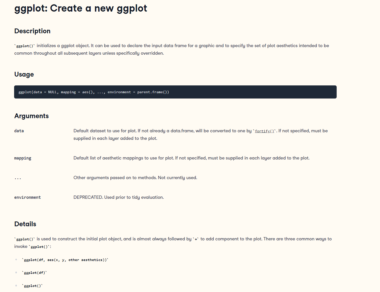{fig-alt="The help page of the ggplot() function." fig-width="175%"}
## Data
```{r}
#| label: setup-ggplot-slides
#| include: false
#| purl: false
library(ggplot2)
theme_set(theme_grey(base_size = 14))
```
```{r}
#| label: ggplot-data
#| output-location: column
ggplot(data = bikes)
```
## Aesthetic Mapping(视觉映射):`aes(.)`
<br>
<b class='simple-highlight-grn' style='font-size:2.6rem;'>= link variables to graphical properties</b><br><br>
::: incremental
- positions (`x`, `y`)
- colors (`color`, `fill`)
- shapes (`shape`, `linetype`)
- size (`size`)
- transparency (`alpha`)
- groupings (`group`)
:::
## Aesthetic Mapping(视觉映射):`aes(.)`
```{r}
#| label: ggplot-aesthetics-outside
#| output-location: column
#| code-line-numbers: "2|1,2"
ggplot(data = bikes) +
aes(x = temp_feel, y = count)
```
## <span style='color:#4758AB;'>aes</span>thetics
`aes()` outside as component
```{r}
#| label: ggplot-aesthetics-outside-comp
#| eval: false
ggplot(data = bikes) +
aes(x = temp_feel, y = count)
```
<br>
::: fragment
`aes()` inside, explicit matching
```{r}
#| label: ggplot-aesthetics-inside
#| eval: false
ggplot(data = bikes, mapping = aes(x = temp_feel, y = count))
```
<br>
:::
::: fragment
`aes()` inside, implicit matching
```{r}
#| label: ggplot-aesthetics-inside-implicit
#| eval: false
ggplot(bikes, aes(temp_feel, count))
```
<br>
:::
::: fragment
`aes()` inside, mixed matching
```{r}
#| label: ggplot-aesthetics-inside-mix
#| eval: false
ggplot(bikes, aes(x = temp_feel, y = count))
```
:::
# Geometrical Layers
## Geometries(几何图层):geom_*
<br>
<b class='simple-highlight-grn' style='font-size:2.6rem;'>= interpret aesthetics as graphical representations</b><br><br>
::: incremental
- points
- lines
- polygons
- text labels
- ...
:::
## Geometries(几何图层):geom_*
```{r}
#| label: geom-point
#| output-location: column
#| code-line-numbers: "1,2,3,4|5"
ggplot(
bikes,
aes(x = temp_feel, y = count)
) +
geom_point()
```
## Visual Properties of Layers(图层属性)
```{r}
#| label: geom-point-properties
#| output-location: column
#| code-line-numbers: "5,6,7,8,9,10,11|6,7,8,9,10"
ggplot(
bikes,
aes(x = temp_feel, y = count)
) +
geom_point(
color = "#28a87d",
alpha = .5,
shape = "X",
stroke = 1,
size = 4
)
```
## Setting vs Mapping of Visual Properties
::: {layout-ncol="2"}
```{r}
#| label: geom-point-properties-set
#| fig-height: 3.5
#| code-line-numbers: "6"
ggplot(
bikes,
aes(x = temp_feel, y = count)
) +
geom_point(
color = "#28a87d",
alpha = .5
)
```
::: fragment
```{r}
#| label: geom-point-properties-map
#| fig-height: 3.5
#| code-line-numbers: "6"
ggplot(
bikes,
aes(x = temp_feel, y = count)
) +
geom_point(
aes(color = season),
alpha = .5
)
```
:::
:::
## Mapping Expressions
```{r}
#| label: geom-point-aes-expression
#| output-location: column
#| code-line-numbers: "6"
ggplot(
bikes,
aes(x = temp_feel, y = count)
) +
geom_point(
aes(color = temp_feel > 20),
alpha = .5
)
```
## Filter Data
```{r}
#| label: geom-point-aes-expression-exercise-na
#| output-location: column
#| code-line-numbers: "2"
ggplot(
filter(bikes, !is.na(weather_type)),
aes(x = temp, y = temp_feel)
) +
geom_point(
aes(color = weather_type == "clear",
size = count),
shape = 18,
alpha = .5
)
```
## Filter Data
```{r}
#| label: geom-point-aes-expression-exercise-na-pipe
#| output-location: column
#| code-line-numbers: "2"
ggplot(
bikes %>% filter(!is.na(weather_type)),
aes(x = temp, y = temp_feel)
) +
geom_point(
aes(color = weather_type == "clear",
size = count),
shape = 18,
alpha = .5
)
```
```{r}
#| label: reset-theme
#| include: false
#| purl: false
theme_set(theme_grey(base_size = 14))
```
## Local vs. Global(应用至当前图层或所有图层)
::: {layout-ncol="2"}
```{r}
#| label: geom-point-aes-geom
#| code-line-numbers: "3,6"
#| fig-height: 3.2
ggplot(
bikes,
aes(x = temp_feel, y = count)
) +
geom_point(
aes(color = season),
alpha = .5
)
```
::: fragment
```{r}
#| label: geom-point-aes-global
#| code-line-numbers: "3,4"
#| fig-height: 3.2
ggplot(
bikes,
aes(x = temp_feel, y = count,
color = season)
) +
geom_point(
alpha = .5
)
```
:::
:::
## Adding More Layers
```{r}
#| label: geom-smooth
#| output-location: column
#| code-line-numbers: "9,10,11"
ggplot(
bikes,
aes(x = temp_feel, y = count,
color = season)
) +
geom_point(
alpha = .5
) +
geom_smooth(
method = "lm"
)
```
## Global Color Encoding
```{r}
#| label: geom-smooth-aes-global
#| output-location: column
#| code-line-numbers: "3,4,9,10,11"
ggplot(
bikes,
aes(x = temp_feel, y = count,
color = season)
) +
geom_point(
alpha = .5
) +
geom_smooth(
method = "lm"
)
```
## Local Color Encoding
```{r}
#| label: geom-smooth-aes-fixed
#| output-location: column
#| code-line-numbers: "6,9,10,11"
ggplot(
bikes,
aes(x = temp_feel, y = count)
) +
geom_point(
aes(color = season),
alpha = .5
) +
geom_smooth(
method = "lm"
)
```
## The \`group\` Aesthetic
```{r}
#| label: geom-smooth-aes-grouped
#| output-location: column
#| code-line-numbers: "10"
ggplot(
bikes,
aes(x = temp_feel, y = count)
) +
geom_point(
aes(color = season),
alpha = .5
) +
geom_smooth(
aes(group = day_night),
method = "lm"
)
```
## Set Both as Global Aesthetics
```{r}
#| label: geom-smooth-aes-global-grouped
#| output-location: column
#| code-line-numbers: "4,5"
ggplot(
bikes,
aes(x = temp_feel, y = count,
color = season,
group = day_night)
) +
geom_point(
alpha = .5
) +
geom_smooth(
method = "lm"
)
```
## Overwrite Global Aesthetics
```{r}
#| label: geom-smooth-aes-global-grouped-overwrite
#| output-location: column
#| code-line-numbers: "4,12"
ggplot(
bikes,
aes(x = temp_feel, y = count,
color = season,
group = day_night)
) +
geom_point(
alpha = .5
) +
geom_smooth(
method = "lm",
color = "black"
)
```
# Statistical Layers
## \`stat_\*()\` and \`geom_\*()\`
::: {layout-ncol="2"}
```{r}
#| label: stat-geom
#| fig-height: 5.1
#| code-line-numbers: "2"
ggplot(bikes, aes(x = temp_feel, y = count)) +
stat_smooth(geom = "smooth")
```
```{r}
#| label: geom-stat
#| fig-height: 5.1
#| code-line-numbers: "2"
ggplot(bikes, aes(x = temp_feel, y = count)) +
geom_smooth(stat = "smooth")
```
:::
## \`stat_\*()\` and \`geom_\*()\`
::: {layout-ncol="2"}
```{r}
#| label: stat-geom-2
#| fig-height: 5.1
#| code-line-numbers: "2"
ggplot(bikes, aes(x = season)) +
stat_count(geom = "bar")
```
```{r}
#| label: geom-stat-2
#| fig-height: 5.1
#| code-line-numbers: "2"
ggplot(bikes, aes(x = season)) +
geom_bar(stat = "count")
```
:::
## \`stat_\*()\` and \`geom_\*()\`
::: {layout-ncol="2"}
```{r}
#| label: stat-geom-3
#| fig-height: 5.1
#| code-line-numbers: "2"
ggplot(bikes, aes(x = date, y = temp_feel)) +
stat_identity(geom = "point")
```
```{r}
#| label: geom-stat-3
#| fig-height: 5.1
#| code-line-numbers: "2"
ggplot(bikes, aes(x = date, y = temp_feel)) +
geom_point(stat = "identity")
```
:::
## Statistical Summaries
```{r}
#| label: stat-summary
#| output-location: column
#| code-line-numbers: "5|3"
ggplot(
bikes,
aes(x = season, y = temp_feel)
) +
stat_summary()
```
## Statistical Summaries
```{r}
#| label: stat-summary-defaults
#| output-location: column
#| code-line-numbers: "6,7"
ggplot(
bikes,
aes(x = season, y = temp_feel)
) +
stat_summary(
fun.data = mean_se, ## the default
geom = "pointrange" ## the default
)
```
## Statistical Summaries
```{r}
#| label: stat-summary-median
#| output-location: column
#| code-line-numbers: "5|5,6,11|6,7,8,9,10,11|7,8"
ggplot(
bikes,
aes(x = season, y = temp_feel)
) +
geom_boxplot() +
stat_summary(
fun = mean,
geom = "point",
color = "#28a87d",
size = 3
)
```
## Statistical Summaries
```{r}
#| label: stat-summary-custom
#| output-location: column
#| code-line-numbers: "5,6,7,8,9|7,8"
ggplot(
bikes,
aes(x = season, y = temp_feel)
) +
stat_summary(
fun = mean,
fun.max = function(y) mean(y) + sd(y),
fun.min = function(y) mean(y) - sd(y)
)
```
# Extending a ggplot
## Store a ggplot as Object
```{r}
#| label: ggplot-object
#| code-line-numbers: "1,16"
g <-
ggplot(
bikes,
aes(x = temp_feel, y = count,
color = season,
group = day_night)
) +
geom_point(
alpha = .5
) +
geom_smooth(
method = "lm",
color = "black"
)
class(g)
```
## Inspect a ggplot Object
```{r}
#| label: ggplot-object-data
g$data
```
## Inspect a ggplot Object
```{r}
#| label: ggplot-object-mapping
g$mapping
```
## Extend a ggplot Object: Add Layers
```{r}
#| label: ggplot-object-extend-geom
#| output-location: column
g +
geom_rug(
alpha = .2
)
```
## Remove a Layer from the Legend
```{r}
#| label: geom-guide-none
#| output-location: column
#| code-line-numbers: "4"
g +
geom_rug(
alpha = .2,
show.legend = FALSE
)
```
## Extend a ggplot Object: Add Labels
```{r}
#| label: ggplot-labs-individual
#| output-location: column
#| code-line-numbers: "2,3,4"
g +
xlab("Feels-like temperature (°F)") +
ylab("Reported bike shares") +
ggtitle("TfL bike sharing trends")
```
## Extend a ggplot Object: Add Labels
```{r}
#| label: ggplot-labs-bundled
#| output-location: column
#| code-line-numbers: "2,3,4,5,6"
g +
labs(
x = "Feels-like temperature (°F)",
y = "Reported bike shares",
title = "TfL bike sharing trends"
)
```
## Extend a ggplot Object: Add Labels
```{r}
#| label: ggplot-labs-bundled-color
#| output-location: column
#| code-line-numbers: "6"
g <- g +
labs(
x = "Feels-like temperature (°F)",
y = "Reported bike shares",
title = "TfL bike sharing trends",
color = "Season:"
)
g
```
## Extend a ggplot Object: Add Labels
```{r}
#| label: ggplot-labs-bundled-extended
#| output-location: column
#| code-line-numbers: "6,7,9"
g +
labs(
x = "Feels-like temperature (°F)",
y = "Reported bike shares",
title = "TfL bike sharing trends",
subtitle = "Reported bike rents versus feels-like temperature in London",
caption = "Data: TfL",
color = "Season:",
tag = "Fig. 1"
)
```
## Extend a ggplot Object: Add Labels
::: {layout-ncol="2"}
```{r}
#| label: ggplot-labs-empty-vs-null-A
#| fig-height: 3.6
#| code-line-numbers: "3"
g +
labs(
x = "",
caption = "Data: TfL"
)
```
```{r}
#| label: ggplot-labs-empty-vs-null-B
#| fig-height: 3.6
#| code-line-numbers: "3"
g +
labs(
x = NULL,
caption = "Data: TfL"
)
```
:::
## Extend a ggplot Object: Themes
::: {layout-ncol="2"}
```{r}
#| label: ggplot-object-extend-theme-light
#| fig-height: 5.5
g + theme_light()
```
::: fragment
```{r}
#| label: ggplot-object-extend-theme-minimal
#| fig-height: 5.5
g + theme_minimal()
```
:::
:::
## Change the Theme Base Settings
```{r}
#| label: ggplot-theme-extend-theme-base
#| output-location: column
#| code-line-numbers: "2,3|1,2,3,4"
g + theme_light(
base_size = 14
)
```
## Set a Theme Globally
```{r}
#| label: ggplot-theme-global
#| output-location: column
theme_set(theme_light())
g
```
## Change the Theme Base Settings
```{r}
#| label: ggplot-theme-global-base
#| output-location: column
#| code-line-numbers: "2,3|1,2,3,4"
theme_set(theme_light(
base_size = 14
))
g
```
## Overwrite Specific Theme Settings
```{r}
#| label: ggplot-theme-settings-individual-1
#| output-location: column
#| code-line-numbers: "2|3"
g +
theme(
panel.grid.minor = element_blank()
)
```
## Overwrite Specific Theme Settings
```{r}
#| label: ggplot-theme-settings-individual-2
#| output-location: column
#| code-line-numbers: "4"
g +
theme(
panel.grid.minor = element_blank(),
plot.title = element_text(face = "bold")
)
```
## Overwrite Specific Theme Settings
```{r}
#| label: ggplot-theme-settings-individual-3
#| output-location: column
#| code-line-numbers: "5"
g +
theme(
panel.grid.minor = element_blank(),
plot.title = element_text(face = "bold"),
legend.position = "top"
)
```
## Overwrite Specific Theme Settings
```{r}
#| label: ggplot-theme-settings-individual-legend-none
#| output-location: column
#| code-line-numbers: "5"
g +
theme(
panel.grid.minor = element_blank(),
plot.title = element_text(face = "bold"),
legend.position = "none"
)
```
## Overwrite Specific Theme Settings
```{r}
#| label: ggplot-theme-settings-individual-4
#| output-location: column
#| code-line-numbers: "6|2,3,4,6,7"
g +
theme(
panel.grid.minor = element_blank(),
plot.title = element_text(face = "bold"),
legend.position = "top",
plot.title.position = "plot"
)
```
## Overwrite Theme Settings Globally
```{r}
#| label: ggplot-theme-settings-global
#| output-location: column
#| code-line-numbers: "1|2,3,4,5|1,2,3,4,5,6"
theme_update(
panel.grid.minor = element_blank(),
plot.title = element_text(face = "bold"),
legend.position = "top",
plot.title.position = "plot"
)
g
```
## Save the Graphic
```{r}
#| label: ggplot-save
#| eval: false
ggsave(g, filename = "my_plot.png")
```
::: fragment
```{r}
#| label: ggplot-save-implicit
#| eval: false
ggsave("my_plot.png")
```
:::
::: fragment
```{r}
#| label: ggplot-save-aspect
#| eval: false
ggsave("my_plot.png", width = 8, height = 5, dpi = 600)
```
:::
::: fragment
```{r}
#| label: ggplot-save-vector
#| eval: false
ggsave("my_plot.pdf", width = 20, height = 12, unit = "cm", device = cairo_pdf)
```
:::
::: fragment
```{r}
#| label: ggplot-save-cairo_pdf
#| eval: false
grDevices::cairo_pdf("my_plot.pdf", width = 10, height = 7)
g
dev.off()
```
:::
------------------------------------------------------------------------
<br>
{fig-alt="A comparison of vector and raster graphics." fig-width="150%"}
# Facets(面)
## Facets(面)
<br>
<b class='simple-highlight-grn' style='font-size:2.6rem;'>= split variables to multiple panels</b><br><br>
::: fragment
Facets are also known as:
- small multiples
- trellis graphs
- lattice plots
- conditioning
:::
------------------------------------------------------------------------
::: {layout-ncol="2"}
```{r}
#| label: facet-types-wrap
#| echo: false
#| purl: false
ggplot(bikes, aes(x = 1, y = 1)) +
geom_text(
aes(label = paste0("Subset for\n", stringr::str_to_title(season))),
size = 5, family = "Cabinet Grotesk", lineheight = .9
) +
facet_wrap(~stringr::str_to_title(season)) +
ggtitle("facet_wrap()") +
theme_bw(base_size = 24) +
theme(
plot.title = element_text(hjust = .5, family = "Tabular", face = "bold"),
strip.text = element_text(face = "bold", size = 18),
panel.grid = element_blank(),
axis.ticks = element_blank(),
axis.text = element_blank(),
axis.title = element_blank(),
plot.background = element_rect(color = "#f8f8f8", fill = "#f8f8f8"),
plot.margin = margin(t = 3, r = 25)
)
```
::: fragment
```{r}
#| label: facet-types-grid
#| echo: false
#| purl: false
data <- tibble(
x = 1, y = 1,
day_night = c("Day", "Day", "Night", "Night"),
year = factor(c("2015", "2016", "2015", "2016"), levels = levels(bikes$year)),
label = c("Subset for\nDay × 2015", "Subset for\nDay × 2016",
"Subset for\nNight × 2015", "Subset for\nNight × 2016")
)
ggplot(data, aes(x = 1, y = 1)) +
geom_text(
aes(label = label),
size = 5, family = "Cabinet Grotesk", lineheight = .9
) +
facet_grid(day_night ~ year) +
ggtitle("facet_grid()") +
theme_bw(base_size = 24) +
theme(
plot.title = element_text(hjust = .5, family = "Tabular", face = "bold"),
strip.text = element_text(face = "bold", size = 18),
panel.grid = element_blank(),
axis.ticks = element_blank(),
axis.text = element_blank(),
axis.title = element_blank(),
plot.background = element_rect(color = "#f8f8f8", fill = "#f8f8f8"),
plot.margin = margin(t = 3, l = 25)
)
```
:::
:::
## Setup
```{r}
#| label: theme-size-facets
#| include: false
#| purl: false
theme_set(theme_light(base_size = 12))
theme_update(
panel.grid.minor = element_blank(),
plot.title = element_text(face = "bold"),
legend.position = "top",
plot.title.position = "plot"
)
```
```{r}
#| label: facet-setup
#| output-location: column
#| code-line-numbers: "1,2,3,4,5,6,7,8,9,10|12"
g <-
ggplot(
bikes,
aes(x = temp_feel, y = count,
color = season)
) +
geom_point(
alpha = .3,
guide = "none"
)
g
```
## Wrapped Facets
```{r}
#| label: facet-wrap
#| output-location: column
#| code-line-numbers: "1,2,3,4|2,4|3"
g +
facet_wrap(
vars(day_night)
)
```
## Wrapped Facets
```{r}
#| label: facet-wrap-circumflex
#| output-location: column
#| code-line-numbers: "3"
g +
facet_wrap(
~ day_night
)
```
## Facet Multiple Variables
```{r}
#| label: facet-wrap-multiple
#| output-location: column
#| code-line-numbers: "3"
g +
facet_wrap(
~ is_workday + day_night
)
```
## Facet Options: Cols + Rows
```{r}
#| label: facet-wrap-options-ncol
#| output-location: column
#| code-line-numbers: "4"
g +
facet_wrap(
~ day_night,
ncol = 1
)
```
## Facet Options: Free Scaling
```{r}
#| label: facet-wrap-options-scales
#| output-location: column
#| code-line-numbers: "5"
g +
facet_wrap(
~ day_night,
ncol = 1,
scales = "free"
)
```
## Facet Options: Free Scaling
```{r}
#| label: facet-wrap-options-freey
#| output-location: column
#| code-line-numbers: "5"
g +
facet_wrap(
~ day_night,
ncol = 1,
scales = "free_y"
)
```
## Facet Options: Switch Labels
```{r}
#| label: facet-wrap-options-switch
#| output-location: column
#| code-line-numbers: "5"
g +
facet_wrap(
~ day_night,
ncol = 1,
switch = "x"
)
```
## Gridded Facets
```{r}
#| label: facet-grid
#| output-location: column
#| code-line-numbers: "2,5|3,4"
g +
facet_grid(
rows = vars(day_night),
cols = vars(is_workday)
)
```
## Gridded Facets
```{r}
#| label: facet-grid-circumflex
#| output-location: column
#| code-line-numbers: "3"
g +
facet_grid(
day_night ~ is_workday
)
```
## Facet Multiple Variables
```{r}
#| label: facet-grid-multiple
#| output-location: column
#| code-line-numbers: "3"
g +
facet_grid(
day_night ~ is_workday + season
)
```
## Facet Options: Free Scaling
```{r}
#| label: facet-grid-options-scales
#| output-location: column
#| code-line-numbers: "4"
g +
facet_grid(
day_night ~ is_workday,
scales = "free"
)
```
## Facet Options: Switch Labels
```{r}
#| label: facet-grid-options-switch
#| output-location: column
#| code-line-numbers: "5"
g +
facet_grid(
day_night ~ is_workday,
scales = "free",
switch = "y"
)
```
## Facet Options: Proportional Spacing
```{r}
#| label: facet-grid-options-space
#| output-location: column
#| code-line-numbers: "4,5|5"
g +
facet_grid(
day_night ~ is_workday,
scales = "free",
space = "free"
)
```
## Facet Options: Proportional Spacing
```{r}
#| label: facet-grid-options-space-y
#| output-location: column
#| code-line-numbers: "4,5"
g +
facet_grid(
day_night ~ is_workday,
scales = "free_y",
space = "free_y"
)
```
## Diamonds Facet
```{r}
#| label: diamonds-facet-start
#| output-location: column
#| code-line-numbers: "1,2,3,4,5,6,7,8,9,10,11,12|8,9,10"
ggplot(
diamonds,
aes(x = carat, y = price)
) +
geom_point(
alpha = .3
) +
geom_smooth(
method = "lm",
se = FALSE,
color = "dodgerblue"
)
```
## Diamonds Facet
```{r}
#| label: diamonds-facet
#| output-location: column
#| code-line-numbers: "13,14,15,16,17"
ggplot(
diamonds,
aes(x = carat, y = price)
) +
geom_point(
alpha = .3
) +
geom_smooth(
method = "lm",
se = FALSE,
color = "dodgerblue"
) +
facet_grid(
cut ~ clarity,
space = "free_x",
scales = "free_x"
)
```
## Diamonds Facet (Dark Theme Bonus)
```{r}
#| label: diamonds-facet-dark
#| output-location: column
#| code-line-numbers: "19,20,21,22"
ggplot(
diamonds,
aes(x = carat, y = price)
) +
geom_point(
alpha = .3,
color = "white"
) +
geom_smooth(
method = "lm",
se = FALSE,
color = "dodgerblue"
) +
facet_grid(
cut ~ clarity,
space = "free_x",
scales = "free_x"
) +
theme_dark(
base_size = 14
)
```
# Scales(尺度)
```{r}
#| label: theme-size-reset
#| include: false
#| purl: false
theme_set(theme_light(base_size = 14))
theme_update(
panel.grid.minor = element_blank(),
plot.title = element_text(face = "bold"),
legend.position = "top",
plot.title.position = "plot"
)
```
## Scales
<br>
<b class='simple-highlight-grn' style='font-size:2.6rem;'>= translate between variable ranges and property ranges</b><br><br>
::: incremental
- feels-like temperature ⇄ x
- reported bike shares ⇄ y
- season ⇄ color
- year ⇄ shape
- ...
:::
## Scales
The `scale_*()` components control the properties of all the<br><b class='simple-highlight-ylw'>aesthetic dimensions mapped to the data.</b>
<br>Consequently, there are `scale_*()` functions for all aesthetics such as:
- **positions** via `scale_x_*()` and `scale_y_*()`
- **colors** via `scale_color_*()` and `scale_fill_*()`
- **sizes** via `scale_size_*()` and `scale_radius_*()`
- **shapes** via `scale_shape_*()` and `scale_linetype_*()`
- **transparency** via `scale_alpha_*()`
## Scales
The `scale_*()` components control the properties of all the<br><b class='simple-highlight-ylw'>aesthetic dimensions mapped to the data.</b>
<br>The extensions (`*`) can be filled by e.g.:
- `continuous()`, `discrete()`, `reverse()`, `log10()`, `sqrt()`, `date()` for positions
- `continuous()`, `discrete()`, `manual()`, `gradient()`, `gradient2()`, `brewer()` for colors
- `continuous()`, `discrete()`, `manual()`, `ordinal()`, `area()`, `date()` for sizes
- `continuous()`, `discrete()`, `manual()`, `ordinal()` for shapes
- `continuous()`, `discrete()`, `manual()`, `ordinal()`, `date()` for transparency
------------------------------------------------------------------------
](../../img/concepts/continuous_discrete.png){fig-size="120%" fig-align="center" fig-alt="Allison Horsts illustration ofthe correct use of continuous versus discrete; however, in {ggplot2} these are interpeted in a different way: as quantitative and qualitative."}
## Continuous vs. Discrete in {ggplot2}
::: {layout-ncol="2"}
## Continuous:<br>quantitative or numerical data
- height
- weight
- age
- counts
## Discrete:<br>qualitative or categorical data
- species
- sex
- study sites
- age group
:::
## Continuous vs. Discrete in {ggplot2}
::: {layout-ncol="2"}
## Continuous:<br>quantitative or numerical data
- height (continuous)
- weight (continuous)
- age (continuous or discrete)
- counts (discrete)
## Discrete:<br>qualitative or categorical data
- species (nominal)
- sex (nominal)
- study site (nominal or ordinal)
- age group (ordinal)
:::
## Aesthetics + Scales
```{r}
#| label: scales-default-invisible
#| output-location: column
#| code-line-numbers: "3,4"
ggplot(
bikes,
aes(x = date, y = count,
color = season)
) +
geom_point()
```
## Aesthetics + Scales
```{r}
#| label: scales-default
#| output-location: column
#| code-line-numbers: "3,4,7,8,9|7,8,9"
ggplot(
bikes,
aes(x = date, y = count,
color = season)
) +
geom_point() +
scale_x_date() +
scale_y_continuous() +
scale_color_discrete()
```
## Scales
```{r}
#| label: scales-overwrite-1
#| output-location: column
#| code-line-numbers: "7"
ggplot(
bikes,
aes(x = date, y = count,
color = season)
) +
geom_point() +
scale_x_continuous() +
scale_y_continuous() +
scale_color_discrete()
```
## Scales
```{r}
#| label: scales-overwrite-2
#| output-location: column
#| code-line-numbers: "8"
ggplot(
bikes,
aes(x = date, y = count,
color = season)
) +
geom_point() +
scale_x_continuous() +
scale_y_log10() +
scale_color_discrete()
```
## Scales
```{r}
#| label: scales-overwrite-3
#| output-location: column
#| code-line-numbers: "9"
ggplot(
bikes,
aes(x = date, y = count,
color = season)
) +
geom_point() +
scale_x_continuous() +
scale_y_log10() +
scale_color_viridis_d()
```
## \`scale_x\|y_continuous\`
```{r}
#| label: scales-xy-continuous-trans
#| output-location: column
#| code-line-numbers: "8,9,10|9"
ggplot(
bikes,
aes(x = date, y = count,
color = season)
) +
geom_point() +
scale_y_continuous(
trans = "log10"
)
```
## \`scale_x\|y_continuous\`
```{r}
#| label: scales-xy-continuous-name
#| output-location: column
#| code-line-numbers: "7,8,9|8"
ggplot(
bikes,
aes(x = date, y = count,
color = season)
) +
geom_point() +
scale_y_continuous(
name = "Reported bike shares"
)
```
## \`scale_x\|y_continuous\`
```{r}
#| label: scales-xy-continuous-breaks-seq
#| output-location: column
#| code-line-numbers: "9"
ggplot(
bikes,
aes(x = date, y = count,
color = season)
) +
geom_point() +
scale_y_continuous(
name = "Reported bike shares",
breaks = seq(0, 60000, by = 15000)
)
```
## \`scale_x\|y_continuous\`
```{r}
#| label: scales-xy-continuous-breaks-short
#| output-location: column
#| code-line-numbers: "9"
ggplot(
bikes,
aes(x = date, y = count,
color = season)
) +
geom_point() +
scale_y_continuous(
name = "Reported bike shares",
breaks = 0:4*15000
)
```
## \`scale_x\|y_continuous\`
```{r}
#| label: scales-xy-continuous-breaks-irregular
#| output-location: column
#| code-line-numbers: "9"
ggplot(
bikes,
aes(x = date, y = count,
color = season)
) +
geom_point() +
scale_y_continuous(
name = "Reported bike shares",
breaks = c(0, 2:12*2500, 40000, 50000)
)
```
## \`scale_x\|y_continuous\`
```{r}
#| label: scales-xy-continuous-labels
#| output-location: column
#| code-line-numbers: "8,10"
ggplot(
bikes,
aes(x = date, y = count,
color = season)
) +
geom_point() +
scale_y_continuous(
name = "Reported bike shares in thousands",
breaks = 0:4*15000,
labels = 0:4*15
)
```
## \`scale_x\|y_continuous\`
```{r}
#| label: scales-xy-continuous-labels-paste
#| output-location: column
#| code-line-numbers: "10"
ggplot(
bikes,
aes(x = date, y = count,
color = season)
) +
geom_point() +
scale_y_continuous(
name = "Reported bike shares in thousands",
breaks = 0:4*15000,
labels = paste(0:4*15000, "bikes")
)
```
## \`scale_x\|y_continuous\`
```{r}
#| label: scales-xy-continuous-limits
#| output-location: column
#| code-line-numbers: "10"
ggplot(
bikes,
aes(x = date, y = count,
color = season)
) +
geom_point() +
scale_y_continuous(
name = "Reported bike shares",
breaks = 0:4*15000,
limits = c(NA, 60000)
)
```
## \`scale_x\|y_continuous\`
```{r}
#| label: scales-xy-continuous-expand.no
#| output-location: column
#| code-line-numbers: "10"
ggplot(
bikes,
aes(x = date, y = count,
color = season)
) +
geom_point() +
scale_y_continuous(
name = "Reported bike shares",
breaks = 0:4*15000,
expand = c(0, 0)
)
```
## \`scale_x\|y_continuous\`
```{r}
#| label: scales-xy-continuous-expand
#| output-location: column
#| code-line-numbers: "10"
ggplot(
bikes,
aes(x = date, y = count,
color = season)
) +
geom_point() +
scale_y_continuous(
name = "Reported bike shares",
breaks = -1:5*15000,
expand = c(.5, .5) ## c(add, mult)
)
```
## \`scale_x\|y_continuous\`
```{r}
#| label: scales-xy-continuous-expand-add-explicit
#| output-location: column
#| code-line-numbers: "10"
ggplot(
bikes,
aes(x = date, y = count,
color = season)
) +
geom_point() +
scale_y_continuous(
name = "Reported bike shares",
breaks = -1:5*15000,
expand = expansion(add = 2000)
)
```
## \`scale_x\|y_continuous\`
```{r}
#| label: scales-xy-continuous-guide-none
#| output-location: column
#| code-line-numbers: "10"
ggplot(
bikes,
aes(x = date, y = count,
color = season)
) +
geom_point() +
scale_y_continuous(
name = "Reported bike shares",
breaks = 0:4*15000,
guide = "none"
)
```
## \`scale_x\|y_date\`
```{r}
#| label: scales-xy-date-breaks-months
#| output-location: column
#| code-line-numbers: "7,10|7,8,9,10|9"
ggplot(
bikes,
aes(x = date, y = count,
color = season)
) +
geom_point() +
scale_x_date(
name = NULL,
date_breaks = "4 months"
)
```
## \`scale_x\|y_date\`
```{r}
#| label: scales-xy-date-breaks-weeks
#| output-location: column
#| code-line-numbers: "9"
ggplot(
bikes,
aes(x = date, y = count,
color = season)
) +
geom_point() +
scale_x_date(
name = NULL,
date_breaks = "20 weeks"
)
```
## \`scale_x\|y_date\` with \`strftime()\`
```{r}
#| label: scales-xy-date-labels
#| output-location: column
#| code-line-numbers: "9,10"
ggplot(
bikes,
aes(x = date, y = count,
color = season)
) +
geom_point() +
scale_x_date(
name = NULL,
date_breaks = "6 months",
date_labels = "%Y/%m/%d"
)
```
## \`scale_x\|y_date\` with \`strftime()\`
```{r}
#| label: scales-xy-date-labels-special
#| output-location: column
#| code-line-numbers: "10"
ggplot(
bikes,
aes(x = date, y = count,
color = season)
) +
geom_point() +
scale_x_date(
name = NULL,
date_breaks = "6 months",
date_labels = "%b '%y"
)
```
## \`scale_x\|y_discrete\`
```{r}
#| label: scales-xy-discrete
#| output-location: column
#| code-line-numbers: "3,6,9|6,7,8,9|7,8"
ggplot(
bikes,
aes(x = season, y = count)
) +
geom_boxplot() +
scale_x_discrete(
name = "Period",
labels = c("Dec-Feb", "Mar-May", "Jun-Aug", "Sep-Nov")
)
```
## \`scale_x\|y_discrete\`
```{r}
#| label: scales-xy-discrete-expand
#| output-location: column
#| code-line-numbers: "8"
ggplot(
bikes,
aes(x = season, y = count)
) +
geom_boxplot() +
scale_x_discrete(
name = "Season",
expand = c(.5, 0) ## add, mult
)
```
## Discrete or Continuous?
```{r}
#| label: scales-xy-fake-discrete-visible
#| output-location: column
#| code-line-numbers: "3,5,6,7"
ggplot(
bikes,
aes(x = as.numeric(season), y = count)
) +
geom_boxplot(
aes(group = season)
)
```
## Discrete or Continuous?
```{r}
#| label: scales-xy-fake-discrete
#| output-location: column
#| code-line-numbers: "9,10,11,12,13|11|12"
ggplot(
bikes,
aes(x = as.numeric(season),
y = count)
) +
geom_boxplot(
aes(group = season)
) +
scale_x_continuous(
name = "Season",
breaks = 1:4,
labels = levels(bikes$season)
)
```
## Discrete or Continuous?
```{r}
#| label: scales-xy-fake-discrete-shift
#| output-location: column
#| code-line-numbers: "3,4"
ggplot(
bikes,
aes(x = as.numeric(season) +
as.numeric(season) / 8,
y = count)
) +
geom_boxplot(
aes(group = season)
) +
scale_x_continuous(
name = "Season",
breaks = 1:4,
labels = levels(bikes$season)
)
```
## \`scale_color\|fill_discrete\`
```{r}
#| label: scales-color-discrete-type-vector
#| output-location: column
#| code-line-numbers: "7,10|7,8,9,10|8,9"
ggplot(
bikes,
aes(x = date, y = count,
color = season)
) +
geom_point() +
scale_color_discrete(
name = "Season:",
type = c("#69b0d4", "#00CB79", "#F7B01B", "#a78f5f")
)
```
## Inspect Assigned Colors
```{r}
#| label: scales-color-discrete-type-inspect
#| output-location: column
#| code-line-numbers: "1|12|14"
g <- ggplot(
bikes,
aes(x = date, y = count,
color = season)
) +
geom_point() +
scale_color_discrete(
name = "Season:",
type = c("#3ca7d9", "#1ec99b", "#F7B01B", "#bb7e8f")
)
gb <- ggplot_build(g)
gb$data[[1]][c(1:5, 200:205, 400:405), 1:5]
```
## \`scale_color\|fill_discrete\`
```{r}
#| label: scales-color-discrete-type-vector-named
#| output-location: column
#| code-line-numbers: "1,2,3,4,5,6|1,16"
my_colors <- c(
`winter` = "#3c89d9",
`spring` = "#1ec99b",
`summer` = "#F7B01B",
`autumn` = "#a26e7c"
)
ggplot(
bikes,
aes(x = date, y = count,
color = season)
) +
geom_point() +
scale_color_discrete(
name = "Season:",
type = my_colors
)
```
## \`scale_color\|fill_discrete\`
```{r}
#| label: scales-color-discrete-type-vector-named-shuffled
#| output-location: column
#| code-line-numbers: "2,5|1,16"
my_colors_alphabetical <- c(
`autumn` = "#a26e7c",
`spring` = "#1ec99b",
`summer` = "#F7B01B",
`winter` = "#3c89d9"
)
ggplot(
bikes,
aes(x = date, y = count,
color = season)
) +
geom_point() +
scale_color_discrete(
name = "Season:",
type = my_colors_alphabetical
)
```
## \`scale_color\|fill_discrete\`
```{r}
#| label: scales-color-discrete-type-palette
#| output-location: column
#| code-line-numbers: "1|11,12,13"
library(RColorBrewer)
ggplot(
bikes,
aes(x = date, y = count,
color = season)
) +
geom_point() +
scale_color_discrete(
name = "Season:",
type = brewer.pal(
n = 4, name = "Dark2"
)
)
```
## \`scale_color\|fill_manual\`
```{r}
#| label: scales-color-manual-na
#| output-location: column
#| code-line-numbers: "4,9,10"
ggplot(
bikes,
aes(x = date, y = count,
color = weather_type)
) +
geom_point() +
scale_color_manual(
name = "Season:",
values = brewer.pal(n = 6, name = "Pastel1"),
na.value = "black"
)
```
## \`scale_color\|fill_carto_d\`
```{r}
#| label: scales-color-discrete-carto
#| output-location: column
#| code-line-numbers: "7,8,9,10"
ggplot(
bikes,
aes(x = date, y = count,
color = weather_type)
) +
geom_point() +
rcartocolor::scale_color_carto_d(
name = "Season:",
palette = "Pastel",
na.value = "black"
)
```
## Diamonds Facet
```{r}
#| label: diamonds-facet-store
#| output-location: column
#| code-line-numbers: "1|10|20"
facet <-
ggplot(
diamonds,
aes(x = carat, y = price)
) +
geom_point(
alpha = .3
) +
geom_smooth(
aes(color = cut),
method = "lm",
se = FALSE
) +
facet_grid(
cut ~ clarity,
space = "free_x",
scales = "free_x"
)
facet
```
## Diamonds Facet
```{r}
#| label: diamonds-facet-scales-xy
#| output-location: column
facet +
scale_x_continuous(
breaks = 0:5
) +
scale_y_continuous(
limits = c(0, 30000),
breaks = 0:3*10000,
labels = c("$0", "$10,000", "$20,000", "$30,000")
)
```
## Diamonds Facet
```{r}
#| label: diamonds-facet-scales-y-paste-format
#| output-location: column
#| code-line-numbers: "8,9,10,11,12,13,14"
facet +
scale_x_continuous(
breaks = 0:5
) +
scale_y_continuous(
limits = c(0, 30000),
breaks = 0:3*10000,
labels = paste0(
"$", format(
0:3*10000,
big.mark = ",",
trim = TRUE
)
)
)
```
## Diamonds Facet
```{r}
#| label: diamonds-facet-scales-y-function
#| output-location: column
#| code-line-numbers: "8,9,10,11,12,13"
facet +
scale_x_continuous(
breaks = 0:5
) +
scale_y_continuous(
limits = c(0, 30000),
breaks = 0:3*10000,
labels = function(y) paste0(
"$", format(
y, big.mark = ",",
trim = TRUE
)
)
)
```
## Diamonds Facet
```{r}
#| label: diamonds-facet-scales-y-dollar-format
#| output-location: column
#| code-line-numbers: "8"
facet +
scale_x_continuous(
breaks = 0:5
) +
scale_y_continuous(
limits = c(0, 30000),
breaks = 0:3*10000,
labels = scales::dollar_format()
)
```
## Diamonds Facet
```{r}
#| label: diamonds-facet-scales-color
#| output-location: column
#| code-line-numbers: "10,11,12,13"
facet +
scale_x_continuous(
breaks = 0:5
) +
scale_y_continuous(
limits = c(0, 30000),
breaks = 0:3*10000,
labels = scales::dollar_format()
) +
scale_color_brewer(
palette = "Set2",
guide = "none"
)
```
## Diamonds Facet
```{r}
#| label: diamonds-facet-scales-no-legend
#| output-location: column
#| code-line-numbers: "13,14,15"
facet +
scale_x_continuous(
breaks = 0:5
) +
scale_y_continuous(
limits = c(0, 30000),
breaks = 0:3*10000,
labels = scales::dollar_format()
) +
scale_color_brewer(
palette = "Set2"
) +
theme(
legend.position = "none"
)
```
# Coordinate Systems(投影)
## Coordinate Systems
<br>
<b class='simple-highlight-grn' style='font-size:2.6rem;'>= interpret the position aesthetics</b><br><br>
::: incremental
- **linear coordinate systems:** preserve the geometrical shapes
- `coord_cartesian()`
- `coord_fixed()`
- `coord_flip()`
- **non-linear coordinate systems:** likely change the geometrical shapes
- `coord_polar()`
- `coord_map()` and `coord_sf()`
- `coord_trans()`
:::
## Cartesian Coordinate System
```{r}
#| label: coord-cartesian
#| output-location: column
#| code-line-numbers: "6"
ggplot(
bikes,
aes(x = season, y = count)
) +
geom_boxplot() +
coord_cartesian()
```
## Cartesian Coordinate System
```{r}
#| label: coord-cartesian-zoom
#| output-location: column
#| code-line-numbers: "6,7,8"
ggplot(
bikes,
aes(x = season, y = count)
) +
geom_boxplot() +
coord_cartesian(
ylim = c(NA, 15000)
)
```
## Changing Limits
::: {layout-ncol="2"}
```{r}
#| label: coord-cartesian-ylim
#| fig-height: 3.5
#| code-line-numbers: "6,7,8"
ggplot(
bikes,
aes(x = season, y = count)
) +
geom_boxplot() +
coord_cartesian(
ylim = c(NA, 15000)
)
```
```{r}
#| label: scale-y-limits
#| fig-height: 3.5
#| code-line-numbers: "6,7,8"
ggplot(
bikes,
aes(x = season, y = count)
) +
geom_boxplot() +
scale_y_continuous(
limits = c(NA, 15000)
)
```
:::
## Clipping
```{r}
#| label: coord-clip
#| output-location: column
#| code-line-numbers: "8"
ggplot(
bikes,
aes(x = season, y = count)
) +
geom_boxplot() +
coord_cartesian(
ylim = c(NA, 15000),
clip = "off"
)
```
## Clipping
```{r}
#| label: coord-clip-text
#| output-location: column
#| code-line-numbers: "2,3|6,7,8,9,10|12"
ggplot(
filter(bikes, is_holiday == TRUE),
aes(x = temp_feel, y = count)
) +
geom_point() +
geom_text(
aes(label = season),
nudge_x = .3,
hjust = 0
) +
coord_cartesian(
clip = "off"
)
```
## ... or better use {ggrepel}
```{r}
#| label: coord-clip-text-repel
#| output-location: column
#| code-line-numbers: "6"
ggplot(
filter(bikes, is_holiday == TRUE),
aes(x = temp_feel, y = count)
) +
geom_point() +
ggrepel::geom_text_repel(
aes(label = season),
nudge_x = .3,
hjust = 0
) +
coord_cartesian(
clip = "off"
)
```
## Remove All Padding
```{r}
#| label: coord-expand-off-clip
#| output-location: column
#| code-line-numbers: "7|8"
ggplot(
bikes,
aes(x = temp_feel, y = count)
) +
geom_point() +
coord_cartesian(
expand = FALSE,
clip = "off"
)
```
## Fixed Coordinate System
::: {layout-ncol="2"}
```{r}
#| label: coord-fixed
#| fig-height: 4.2
#| code-line-numbers: "6"
ggplot(
bikes,
aes(x = temp_feel, y = temp)
) +
geom_point() +
coord_fixed()
```
::: fragment
```{r}
#| label: coord-fixed-custom
#| fig-height: 4.2
#| code-line-numbers: "6"
ggplot(
bikes,
aes(x = temp_feel, y = temp)
) +
geom_point() +
coord_fixed(ratio = 4)
```
:::
:::
## Flipped Coordinate System
::: {layout-ncol="2"}
```{r}
#| label: coord-cartesian-comp-flip
#| fig-height: 4.1
#| code-line-numbers: "6"
ggplot(
bikes,
aes(x = weather_type)
) +
geom_bar() +
coord_cartesian()
```
```{r}
#| label: coord-flip
#| fig-height: 4.1
#| code-line-numbers: "6"
ggplot(
bikes,
aes(x = weather_type)
) +
geom_bar() +
coord_flip()
```
:::
## Flipped Coordinate System
::: {layout-ncol="2"}
```{r}
#| label: coord-cartesian-switch-x-y
#| fig-height: 4.1
#| code-line-numbers: "3,6"
ggplot(
bikes,
aes(y = weather_type)
) +
geom_bar() +
coord_cartesian()
```
```{r}
#| label: coord-flip-again
#| fig-height: 4.1
#| code-line-numbers: "3,6"
ggplot(
bikes,
aes(x = weather_type)
) +
geom_bar() +
coord_flip()
```
:::
## Reminder: Sort Your Bars!
```{r}
#| label: forcats-sort-infreq
#| output-location: column
#| code-line-numbers: "3|2"
ggplot(
filter(bikes, !is.na(weather_type)),
aes(y = fct_infreq(weather_type))
) +
geom_bar()
```
## Reminder: Sort Your Bars!
```{r}
#| label: forcats-sort-infreq-rev
#| output-location: column
#| code-line-numbers: "3,4,5"
ggplot(
filter(bikes, !is.na(weather_type)),
aes(y = fct_rev(
fct_infreq(weather_type)
))
) +
geom_bar()
```
## Circular Corrdinate System
::: {layout-ncol="2"}
```{r}
#| label: coord-polar
#| fig-height: 3.9
#| code-line-numbers: "7"
ggplot(
filter(bikes, !is.na(weather_type)),
aes(x = weather_type,
fill = weather_type)
) +
geom_bar() +
coord_polar()
```
::: fragment
```{r}
#| label: coord-cartesian-comp-polar
#| fig-height: 3.9
#| code-line-numbers: "7"
ggplot(
filter(bikes, !is.na(weather_type)),
aes(x = weather_type,
fill = weather_type)
) +
geom_bar() +
coord_cartesian()
```
:::
:::
## Circular Cordinate System
::: {layout-ncol="2"}
```{r}
#| label: coord-polar-coxcomb
#| fig-height: 3.9
#| code-line-numbers: "6,7"
ggplot(
filter(bikes, !is.na(weather_type)),
aes(x = fct_infreq(weather_type),
fill = weather_type)
) +
geom_bar(width = 1) +
coord_polar()
```
```{r}
#| label: coord-cartesian-comp-polar-no-padding
#| fig-height: 3.9
#| code-line-numbers: "6,7"
ggplot(
filter(bikes, !is.na(weather_type)),
aes(x = fct_infreq(weather_type),
fill = weather_type)
) +
geom_bar(width = 1) +
coord_cartesian()
```
:::
## Circular Corrdinate System
::: {layout-ncol="2"}
```{r}
#| label: coord-polar-theta-x
#| fig-height: 3.9
#| code-line-numbers: "7"
ggplot(
filter(bikes, !is.na(weather_type)),
aes(x = fct_infreq(weather_type),
fill = weather_type)
) +
geom_bar() +
coord_polar(theta = "x")
```
```{r}
#| label: coord-polar-theta-y
#| fig-height: 3.9
#| code-line-numbers: "7"
ggplot(
filter(bikes, !is.na(weather_type)),
aes(x = fct_infreq(weather_type),
fill = weather_type)
) +
geom_bar() +
coord_polar(theta = "y")
```
:::
## Circular Corrdinate System
::: {layout-ncol="2"}
```{r}
#| label: coord-polar-pie
#| fig-height: 4.1
#| code-line-numbers: "5"
ggplot(
filter(bikes, !is.na(weather_type)),
aes(x = 1, fill = weather_type)
) +
geom_bar(position = "stack") +
coord_polar(theta = "y")
```
```{r}
#| label: coord-cartesian-comp-polar-stacked
#| fig-height: 4.1
#| code-line-numbers: "5"
ggplot(
filter(bikes, !is.na(weather_type)),
aes(x = 1, fill = weather_type)
) +
geom_bar(position = "stack") +
coord_cartesian()
```
:::
## Circular Corrdinate System
::: {layout-ncol="2"}
```{r}
#| label: coord-polar-pie-sorted
#| fig-height: 3.6
#| code-line-numbers: "4,6,7"
ggplot(
filter(bikes, !is.na(weather_type)),
aes(x = 1,
fill = fct_rev(fct_infreq(weather_type)))
) +
geom_bar(position = "stack") +
coord_polar(theta = "y") +
scale_fill_discrete(name = NULL)
```
```{r}
#| label: coord-cartesian-comp-polar-stacked-sorted
#| fig-height: 3.6
#| code-line-numbers: "4,6,7"
ggplot(
filter(bikes, !is.na(weather_type)),
aes(x = 1,
fill = fct_rev(fct_infreq(weather_type)))
) +
geom_bar(position = "stack") +
coord_cartesian() +
scale_fill_discrete(name = NULL)
```
:::
## Transform a Coordinate System
```{r}
#| label: coord-trans-log
#| output-location: column
#| code-line-numbers: "6"
ggplot(
bikes,
aes(x = temp, y = count)
) +
geom_point() +
coord_trans(y = "log10")
```
## Transform a Coordinate System
::: {layout-ncol="2"}
```{r}
#| label: trans-log-via-coord
#| fig-height: 3.6
#| code-line-numbers: "6"
ggplot(
bikes,
aes(x = temp, y = count,
group = day_night)
) +
geom_point() +
geom_smooth(method = "lm") +
coord_trans(y = "log10")
```
::: fragment
```{r}
#| label: trans-log-via-scale
#| fig-height: 3.6
#| code-line-numbers: "6"
ggplot(
bikes,
aes(x = temp, y = count,
group = day_night)
) +
geom_point() +
geom_smooth(method = "lm") +
scale_y_log10()
```
:::
:::
# 图形组合
------------------------------------------------------------------------
](../../img/layout/ah_patchwork.jpg){fig-align="center" fig-alt="Allison Horsts monster illustration of the patchwork extension package."}
::: footer
:::
------------------------------------------------------------------------
::: panel-tabset
### Graphic
```{r}
#| label: patchwork-p1
#| fig-width: 10
#| fig-height: 5.8
#| echo: false
theme_std <- theme_set(theme_minimal(base_size = 18))
theme_update(
# text = element_text(family = "Pally"),
panel.grid = element_blank(),
axis.text = element_text(color = "grey50", size = 12),
axis.title = element_text(color = "grey40", face = "bold"),
axis.title.x = element_text(margin = margin(t = 12)),
axis.title.y = element_text(margin = margin(r = 12)),
axis.line = element_line(color = "grey80", size = .4),
legend.text = element_text(color = "grey50", size = 12),
plot.tag = element_text(size = 40, margin = margin(b = 15)),
plot.background = element_rect(fill = "white", color = "white")
)
bikes_sorted <-
bikes %>%
filter(!is.na(weather_type)) %>%
group_by(weather_type) %>%
mutate(sum = sum(count)) %>%
ungroup() %>%
mutate(
weather_type = forcats::fct_reorder(
str_to_title(str_wrap(weather_type, 5)), sum
)
)
p1 <- ggplot(
bikes_sorted,
aes(x = weather_type, y = count, color = weather_type)
) +
geom_hline(yintercept = 0, color = "grey80", size = .4) +
stat_summary(
geom = "point", fun = "sum", size = 12
) +
stat_summary(
geom = "linerange", ymin = 0, fun.max = function(y) sum(y),
size = 2, show.legend = FALSE
) +
coord_flip(ylim = c(0, NA), clip = "off") +
scale_y_continuous(
expand = c(0, 0), limits = c(0, 8500000),
labels = scales::comma_format(scale = .0001, suffix = "K")
) +
scale_color_viridis_d(
option = "magma", direction = -1, begin = .1, end = .9, name = NULL,
guide = guide_legend(override.aes = list(size = 7))
) +
labs(
x = NULL, y = "Sum of reported bike shares", tag = "P1",
) +
theme(
axis.line.y = element_blank(),
axis.text.y = element_text(family = "Pally", color = "grey50", face = "bold",
margin = margin(r = 15), lineheight = .9)
)
p1
```
### Code
```{r}
#| label: patchwork-p1
#| eval: false
```
:::
------------------------------------------------------------------------
::: panel-tabset
### Graphic
```{r}
#| label: patchwork-p2
#| fig-width: 10
#| fig-height: 5.8
#| echo: false
p2 <- bikes_sorted %>%
filter(season == "winter", is_weekend == TRUE, day_night == "night") %>%
group_by(weather_type, .drop = FALSE) %>%
mutate(id = row_number()) %>%
ggplot(
aes(x = weather_type, y = id, color = weather_type)
) +
geom_point(size = 4.5) +
scale_color_viridis_d(
option = "magma", direction = -1, begin = .1, end = .9, name = NULL,
guide = guide_legend(override.aes = list(size = 7))
) +
labs(
x = NULL, y = "Reported bike shares on\nweekend winter nights", tag = "P2",
) +
coord_cartesian(ylim = c(.5, NA), clip = "off")
p2
```
### Code
```{r}
#| label: patchwork-p2
#| eval: false
```
:::
------------------------------------------------------------------------
::: panel-tabset
### Graphic
```{r}
#| label: patchwork-p3
#| fig-width: 10
#| fig-height: 5.8
#| echo: false
my_colors <- c("#cc0000", "#000080")
p3 <- bikes %>%
group_by(week = lubridate::week(date), day_night, year) %>%
summarize(count = sum(count)) %>%
group_by(week, day_night) %>%
mutate(avg = mean(count)) %>%
ggplot(aes(x = week, y = count, group = interaction(day_night, year))) +
geom_line(color = "grey65", size = 1) +
geom_line(aes(y = avg, color = day_night), stat = "unique", size = 1.7) +
annotate(
geom = "text", label = c("Day", "Night"), color = my_colors,
x = c(5, 18), y = c(125000, 29000), size = 8, fontface = "bold", family = "Pally"
) +
scale_x_continuous(breaks = c(1, 1:10*5)) +
scale_y_continuous(labels = scales::comma_format()) +
scale_color_manual(values = my_colors, guide = "none") +
labs(
x = "Week of the Year", y = "Reported bike shares\n(cumulative # per week)", tag = "P3",
)
p3
```
### Code
```{r}
#| label: patchwork-p3
#| eval: false
```
:::
## {patchwork}
```{r}
#| label: patchwork-composition
#| fig-width: 15
#| fig-height: 12
#| fig-align: "center"
#| code-line-numbers: "3|2,3"
# install.packages("patchwork")
require(patchwork)
(p1 + p2) / p3
```
## "Collect Guides"
```{r}
#| label: patchwork-composition-guides
#| fig-width: 15
#| fig-height: 12
#| fig-align: "center"
(p1 + p2) / p3 + plot_layout(guides = "collect")
```
## Apply Theming
```{r}
#| label: patchwork-composition-guides-just
#| fig-width: 15
#| fig-height: 12
#| fig-align: "center"
((p1 + p2) / p3 & theme(legend.justification = "top")) +
plot_layout(guides = "collect")
```
## Apply Theming
```{r}
#| label: patchwork-composition-legend-off
#| fig-width: 15
#| fig-height: 12
#| fig-align: "center"
(p1 + p2) / p3 & theme(legend.position = "none",
plot.background = element_rect(color = "black", size = 3))
```
## Adjust Widths and Heights
```{r}
#| label: patchwork-composition-heights-widths
#| fig-width: 15
#| fig-height: 12
#| fig-align: "center"
#| code-line-numbers: "2"
((p1 + p2) / p3 & theme(legend.position = "none")) +
plot_layout(heights = c(.2, .1), widths = c(2, 1))
```
## Use A Custom Layout
```{r}
#| label: patchwork-composition-design
#| fig-width: 15
#| fig-height: 12
#| fig-align: "center"
#| code-line-numbers: "1,2,3,4|5"
picasso <- "
AAAAAA#BBBB
CCCCCCCCC##
CCCCCCCCC##"
(p1 + p2 + p3 & theme(legend.position = "none")) +
plot_layout(design = picasso)
```
## Add Labels
```{r}
#| label: patchwork-composition-labs-prep
pl1 <- p1 + labs(tag = NULL, title = "Plot One") + theme(legend.position = "none")
pl2 <- p2 + labs(tag = NULL, title = "Plot Two") + theme(legend.position = "none")
pl3 <- p3 + labs(tag = NULL, title = "Plot Three") + theme(legend.position = "none")
```
## Add Labels
```{r}
#| label: patchwork-composition-labs
#| fig-width: 15
#| fig-height: 12
#| fig-align: "center"
#| code-line-numbers: "2"
(pl1 + pl2) / pl3 +
plot_annotation(tag_levels = "1",
tag_prefix = "P",
title = "An overarching title for all 3 plots, placed on the very top while all other titles are sitting below the tags.")
```
## Add Text
::: panel-tabset
### Graphic
```{r}
#| label: patchwork-composition-textbox-prep
#| echo: false
#| fig-width: 9
#| fig-height: 4.5
#| fig-align: "center"
text <- tibble::tibble(
x = 0, y = 0, label = "Lorem ipsum dolor sit amet, **consectetur adipiscing elit**, sed do eiusmod tempor incididunt ut labore et dolore magna aliqua. Ut enim ad minim veniam, quis nostrud exercitation <b style='color:#000080;'>ullamco laboris nisi</b> ut aliquip ex ea commodo consequat. Duis aute irure dolor in reprehenderit in voluptate velit esse cillum dolore eu fugiat nulla pariatur. Excepteur sint occaecat <b style='color:#cc0000;'>cupidatat non proident</b>, sunt in culpa qui officia deserunt mollit anim id est laborum."
)
pt <- ggplot(text, aes(x = x, y = y)) +
ggtext::geom_textbox(
aes(label = label),
box.color = NA, width = unit(23, "lines"),
color = "grey40", size = 6.5, lineheight = 1.4
) +
coord_cartesian(expand = FALSE, clip = "off") +
theme_void()
pt
```
### Code
```{r}
#| label: patchwork-composition-textbox-prep
#| eval: false
```
:::
## Add Text
```{r}
#| label: patchwork-composition-textbox
#| fig-width: 15
#| fig-height: 12
#| fig-align: "center"
(p1 + pt) / p3
```
## Add Inset Plots
```{r}
#| label: patchwork-composition-inset-1
#| fig-width: 12
#| fig-height: 7
#| fig-align: "center"
pl1 + inset_element(pl2,
l = .6, b = .1, r = 1, t = .6)
```
## Add Inset Plots
```{r}
#| label: patchwork-composition-inset-2
#| fig-width: 12
#| fig-height: 7
#| fig-align: "center"
pl1 + inset_element(pl2,
l = .6, b = 0, r = 1, t = .5, align_to = 'full')
```
## Add Inset Plots
```{r}
#| label: patchwork-composition-inset-3
#| fig-width: 15
#| fig-height: 12
#| fig-align: "center"
(pl1 + inset_element(pl2,
l = .6, b = .1, r = 1, t = .6) + pt) / pl3
```
## 练习
```{r}
library(palmerpenguins)
library(ggthemes)
penguins
```
## 效果
```{r}
#| echo: false
#| warning: false
#| fig-width: 8
#| fig-height: 5
penguins |>
ggplot(aes(x = flipper_length_mm, y = body_mass_g)) +
geom_point(aes(color = species, shape = species)) +
geom_smooth(method = "lm") +
labs(
title = "Body mass and flipper length",
subtitle = "Dimensions for Adelie, Chinstrap, and Gentoo Penguins",
x = "Flipper length (mm)",
y = "Body mass (g)",
color = "Species",
shape = "Species"
) +
scale_color_colorblind()
```
```{r}
#| include: false
#| fig-alt: |
#| A blank, gray plot area.
ggplot(data = penguins)
```
```{r}
#| include: false
ggplot(
data = penguins,
mapping = aes(x = flipper_length_mm, y = body_mass_g)
)
```
```{r}
#| include: false
#| fig-alt: |
#| A scatterplot of body mass vs. flipper length of penguins. The plot
#| displays a positive, linear, and relatively strong relationship between
#| these two variables.
ggplot(
data = penguins,
mapping = aes(x = flipper_length_mm, y = body_mass_g)
) +
geom_point()
```
```{r}
#| include: false
#| warning: false
#| fig-alt: |
#| A scatterplot of body mass vs. flipper length of penguins. The plot
#| displays a positive, fairly linear, and relatively strong relationship
#| between these two variables. Species (Adelie, Chinstrap, and Gentoo)
#| are represented with different colors.
ggplot(
data = penguins,
mapping = aes(x = flipper_length_mm, y = body_mass_g, color = species)
) +
geom_point()
```
```{r}
#| include: false
#| warning: false
#| fig-alt: |
#| A scatterplot of body mass vs. flipper length of penguins. Overlaid
#| on the scatterplot are three smooth curves displaying the
#| relationship between these variables for each species (Adelie,
#| Chinstrap, and Gentoo). Different penguin species are plotted in
#| different colors for the points and the smooth curves.
ggplot(
data = penguins,
mapping = aes(x = flipper_length_mm, y = body_mass_g, color = species)
) +
geom_point() +
geom_smooth(method = "lm")
```
```{r}
#| include: false
#| warning: false
#| fig-alt: |
#| A scatterplot of body mass vs. flipper length of penguins. Overlaid
#| on the scatterplot is a single line of best fit displaying the
#| relationship between these variables for each species (Adelie,
#| Chinstrap, and Gentoo). Different penguin species are plotted in
#| different colors for the points only.
ggplot(
data = penguins,
mapping = aes(x = flipper_length_mm, y = body_mass_g)
) +
geom_point(mapping = aes(color = species)) +
geom_smooth(method = "lm")
```
```{r}
#| include: false
#| warning: false
#| fig-alt: |
#| A scatterplot of body mass vs. flipper length of penguins. Overlaid
#| on the scatterplot is a single line of best fit displaying the
#| relationship between these variables for each species (Adelie,
#| Chinstrap, and Gentoo). Different penguin species are plotted in
#| different colors and shapes for the points only.
ggplot(
data = penguins,
mapping = aes(x = flipper_length_mm, y = body_mass_g)
) +
geom_point(mapping = aes(color = species, shape = species)) +
geom_smooth(method = "lm")
```
## 练习
:::: {.panel-tabset}
### Code
```{r}
p <- ggplot(
data = penguins,
mapping = aes(x = flipper_length_mm, y = body_mass_g)
) +
geom_point(aes(color = species, shape = species)) +
geom_smooth(method = "lm") +
labs(
title = "Body mass and flipper length",
subtitle = "Dimensions for Adelie, Chinstrap, and Gentoo Penguins",
x = "Flipper length (mm)", y = "Body mass (g)",
color = "Species", shape = "Species"
) +
scale_color_colorblind()
```
### Graphic
```{r}
#| echo: false
#| fig-width: 8
#| fig-height: 5
p
```
::::
## 练习
:::: {.panel-tabset}
### Code
```{r}
#| warning: false
#| fig-alt: |
#| A scatterplot of body mass vs. flipper length of penguins, colored
#| by bill depth. A smooth curve of the relationship between body mass
#| and flipper length is overlaid. The relationship is positive,
#| fairly linear, and moderately strong.
p <- ggplot(
data = penguins,
mapping = aes(x = flipper_length_mm, y = body_mass_g)) +
geom_point(aes(color = bill_depth_mm)) +
geom_smooth()
```
### Graphic
```{r}
#| echo: false
#| fig-width: 8
#| fig-height: 5
p
```
::::
## 练习
:::: {.panel-tabset}
### Code
```{r}
p <- ggplot(
data = penguins,
mapping = aes(x = flipper_length_mm, y = body_mass_g, color = island)
) +
geom_point() +
geom_smooth(se = FALSE)
```
### Graphic
```{r}
#| echo: false
#| fig-width: 8
#| fig-height: 5
p
```
::::
## 分层展示
:::: {.panel-tabset}
### Code
```{r}
p <- ggplot(
data = penguins,
mapping = aes(x = flipper_length_mm, y = body_mass_g)
) +
geom_point() +
geom_smooth()
```
### Graphic
```{r}
#| echo: false
#| fig-width: 8
#| fig-height: 5
p
```
::::
## 柱状图
:::: {.panel-tabset}
### Code
```{r}
#| fig-alt: |
#| A bar chart of frequencies of species of penguins: Adelie
#| (approximately 150), Chinstrap (approximately 90), Gentoo
#| (approximately 125).
p <- ggplot(penguins, aes(x = species)) +
geom_bar()
```
### Graphic
```{r}
#| echo: false
#| fig-width: 8
#| fig-height: 5
p
```
::::
## 柱状图
:::: {.panel-tabset}
### Code
```{r}
#| fig-alt: |
#| A bar chart of frequencies of species of penguins, where the bars are
#| ordered in decreasing order of their heights (frequencies): Adelie
#| (approximately 150), Gentoo (approximately 125), Chinstrap
#| (approximately 90).
p <- ggplot(penguins, aes(x = fct_infreq(species))) +
geom_bar()
```
### Graphic
```{r}
#| echo: false
#| fig-width: 8
#| fig-height: 5
p
```
::::
## 直方图
:::: {.panel-tabset}
### Code
```{r}
#| warning: false
#| fig-alt: |
#| A histogram of body masses of penguins. The distribution is unimodal
#| and right skewed, ranging between approximately 2500 to 6500 grams.
p <- ggplot(penguins, aes(x = body_mass_g)) +
geom_histogram(binwidth = 200)
```
### Graphic
```{r}
#| echo: false
#| fig-width: 8
#| fig-height: 5
p
```
::::
## 直方图
:::: {.panel-tabset}
### Code
```{r}
#| warning: false
#| layout-ncol: 2
#| fig-width: 3
#| fig-alt: |
#| Two histograms of body masses of penguins, one with binwidth of 20
#| (left) and one with binwidth of 2000 (right). The histogram with binwidth
#| of 20 shows lots of ups and downs in the heights of the bins, creating a
#| jagged outline. The histogram with binwidth of 2000 shows only three bins.
p1 <- ggplot(penguins, aes(x = body_mass_g)) +
geom_histogram(binwidth = 20)
p2 <- ggplot(penguins, aes(x = body_mass_g)) +
geom_histogram(binwidth = 2000)
p <- p1 + p2
```
### Graphic
```{r}
#| echo: false
#| fig-width: 10
#| fig-height: 5
p
```
::::
## 密度图
:::: {.panel-tabset}
### Code
```{r}
#| fig-alt: |
#| A density plot of body masses of penguins. The distribution is unimodal
#| and right skewed, ranging between approximately 2500 to 6500 grams.
p <- ggplot(penguins, aes(x = body_mass_g)) +
geom_density()
```
### Graphic
```{r}
#| echo: false
#| fig-width: 8
#| fig-height: 5
p
```
::::
## 箱图
:::: {.panel-tabset}
### Code
```{r}
#| warning: false
#| fig-alt: |
#| Side-by-side box plots of distributions of body masses of Adelie,
#| Chinstrap, and Gentoo penguins. The distribution of Adelie and
#| Chinstrap penguins' body masses appear to be symmetric with
#| medians around 3750 grams. The median body mass of Gentoo penguins
#| is much higher, around 5000 grams, and the distribution of the
#| body masses of these penguins appears to be somewhat right skewed.
p <- ggplot(penguins,
aes(x = species, y = body_mass_g)) +
geom_boxplot()
```
### Graphic
```{r}
#| echo: false
#| fig-width: 8
#| fig-height: 5
p
```
::::
## 分组
:::: {.panel-tabset}
### Code
```{r}
#| warning: false
#| fig-alt: |
#| A density plot of body masses of penguins by species of penguins. Each
#| species (Adelie, Chinstrap, and Gentoo) is represented with different
#| colored outlines for the density curves.
p <- ggplot(penguins,
aes(x = body_mass_g, color = species)) +
geom_density(linewidth = 0.75)
```
### Graphic
```{r}
#| echo: false
#| fig-width: 8
#| fig-height: 5
p
```
::::
## 分组
:::: {.panel-tabset}
### Code
```{r}
#| warning: false
#| fig-alt: |
#| A density plot of body masses of penguins by species of penguins. Each
#| species (Adelie, Chinstrap, and Gentoo) is represented in different
#| colored outlines for the density curves. The density curves are also
#| filled with the same colors, with some transparency added.
p <- ggplot(penguins,
aes(x = body_mass_g, color = species, fill = species)) +
geom_density(alpha = 0.5)
```
### Graphic
```{r}
#| echo: false
#| fig-width: 8
#| fig-height: 5
p
```
::::
## 分组
:::: {.panel-tabset}
### Code
```{r}
#| fig-alt: |
#| Bar plots of penguin species by island (Biscoe, Dream, and Torgersen)
p <- ggplot(penguins,
aes(x = island, fill = species)) +
geom_bar()
```
### Graphic
```{r}
#| echo: false
#| fig-width: 8
#| fig-height: 5
p
```
::::
## 分组
:::: {.panel-tabset}
### Code
```{r}
#| fig-alt: |
#| Bar plots of penguin species by island (Biscoe, Dream, and Torgersen)
#| the bars are scaled to the same height, making it a relative frequencies
#| plot
p <- ggplot(penguins,
aes(x = island, fill = species)) +
geom_bar(position = "fill")
```
### Graphic
```{r}
#| echo: false
#| fig-width: 8
#| fig-height: 5
p
```
::::
## 分组
:::: {.panel-tabset}
### Code
```{r}
#| warning: false
#| fig-alt: |
#| A scatterplot of body mass vs. flipper length of penguins. The plot
#| displays a positive, linear, relatively strong relationship between
#| these two variables.
p <- ggplot(penguins,
aes(x = flipper_length_mm, y = body_mass_g)) +
geom_point()
```
### Graphic
```{r}
#| echo: false
#| fig-width: 8
#| fig-height: 5
p
```
::::
## 分组
:::: {.panel-tabset}
### Code
```{r}
#| warning: false
#| fig-alt: |
#| A scatterplot of body mass vs. flipper length of penguins. The plot
#| displays a positive, linear, relatively strong relationship between
#| these two variables. The points are colored based on the species of the
#| penguins and the shapes of the points represent islands (round points are
#| Biscoe island, triangles are Dream island, and squared are Torgersen
#| island). The plot is very busy and it's difficult to distinguish the shapes
#| of the points.
p <- ggplot(penguins,
aes(x = flipper_length_mm, y = body_mass_g)) +
geom_point(aes(color = species, shape = island))
```
### Graphic
```{r}
#| echo: false
#| fig-width: 8
#| fig-height: 5
p
```
::::
## 分面
:::: {.panel-tabset}
### Code
```{r}
#| warning: false
#| fig-width: 8
#| fig-asp: 0.33
#| fig-alt: |
#| A scatterplot of body mass vs. flipper length of penguins. The shapes and
#| colors of points represent species. Penguins from each island are on a
#| separate facet. Within each facet, the relationship between body mass and
#| flipper length is positive, linear, relatively strong.
p <- ggplot(penguins,
aes(x = flipper_length_mm, y = body_mass_g)) +
geom_point(aes(color = species, shape = species)) +
facet_wrap(~island)
```
### Graphic
```{r}
#| echo: false
#| fig-width: 8
#| fig-height: 5
p
```
::::
## 分面
:::: {.panel-tabset}
### Code
```{r}
#| warning: false
p <- ggplot(
data = penguins,
mapping = aes(
x = bill_length_mm, y = bill_depth_mm,
color = species, shape = species
)
) +
geom_point() +
labs(color = "Species")
```
### Graphic
```{r}
#| echo: false
#| fig-width: 8
#| fig-height: 5
p
```
::::
## 练习
:::: {.panel-tabset}
### Code
```{r}
#| layout-ncol: 2
p1 <- ggplot(penguins, aes(x = island, fill = species)) +
geom_bar(position = "fill")
p2 <- ggplot(penguins, aes(x = species, fill = island)) +
geom_bar(position = "fill")
p <- p1 + p2
```
### Graphic
```{r}
#| echo: false
#| fig-width: 10
#| fig-height: 5
p
```
::::
## 练习
:::: {.panel-tabset}
### Code
```{r}
p <- ggplot(penguins,
aes(x = flipper_length_mm, y = body_mass_g)) +
geom_point()
```
### Graphic
```{r}
#| echo: false
#| fig-width: 8
#| fig-height: 5
p
```
::::
## 练习
:::: {.panel-tabset}
### Code
```{r}
p <- ggplot(mpg, aes(x = class)) +
geom_bar()
```
### Graphic
```{r}
#| echo: false
#| fig-width: 8
#| fig-height: 5
p
```
::::
## 练习
:::: {.panel-tabset}
### Code
```{r}
p <- ggplot(mpg, aes(x = cty, y = hwy)) +
geom_point()
```
### Graphic
```{r}
#| echo: false
#| fig-width: 8
#| fig-height: 5
p
```
::::
## 练习
:::: {.panel-tabset}
### Code
```{r}
p <- ggplot(data = mpg) +
geom_point(mapping = aes(x = displ, y = hwy))
```
### Graphic
```{r}
#| echo: false
#| fig-width: 8
#| fig-height: 5
p
```
::::
## 欢迎讨论!{.center}
`r rmdify::slideend(wechat = FALSE, type = "public", tel = FALSE, thislink = "https://drc.drwater.net/course/public/RWEP/PUB/SD/")`